The past few months I’ve used my spare blog energy to work on a fun project that I’d like to loop everyone into!
On August 1st I received an email from the OpenSky listserv (I became a member while building) my Planes Overhead app for the Tidbyt) announcing a data science challenge, focused on predicting plane take off weights. This challenge felt precision targeted for me, as a great lover of planes and machine learning dilettante!
Calling all Data Scientists: Compete in the Eurocontrol PRC Data Challenge!
Together with Eurocontrol’s Performance Review Committee we are announcing a new aviation data challenge! Predict the actual take off weights of aircraft correctly based on their OpenSky data - and win a cumulative 5000 EUR!
I wrapped up my final submission to the challenge a few weeks ago - I don’t think I’ll be winning the five thousand euros, but I had an amazing time building out a (pretty decent!) predictive model and want to give the whole effort some closure with a blog writeup!
The Challenge
The challenge has a great website with documentation on all facets of the competition - I’ve pasted the most important details below as a quick overview:
Goal
The Performance Review Commission (PRC) Data Challenge aims at engaging with data scientists, even without Aviation background, to create teams and compete to build an open Machine Learning (ML) model able to accurately infer the Actual TakeOff Weight (ATOW) of a flown flight.
ATOW is an important input for models estimating fuel burnt and derived gaseous emissions. The current lack of openly available ATOW is typically compensated by assuming it to be equal to a certain percentage of the Maximum TakeOff Weight (MTOW) for the relevant aircraft model. With this challenge we aim at making available a better way to estimate ATOW, i.e. an Estimated TakeOff Weight (ETOW).
The PRC thinks that there is a great pool of Data Scientists that could help to define the open model of the Challenge, but above that, it is the importance to have a white box approach to the way the model is being built. This transparency is a way to build trust, reproducibility and eventually evolve a collaboration to improve the understanding (and the reduction) of the impact of aviation to the environment.
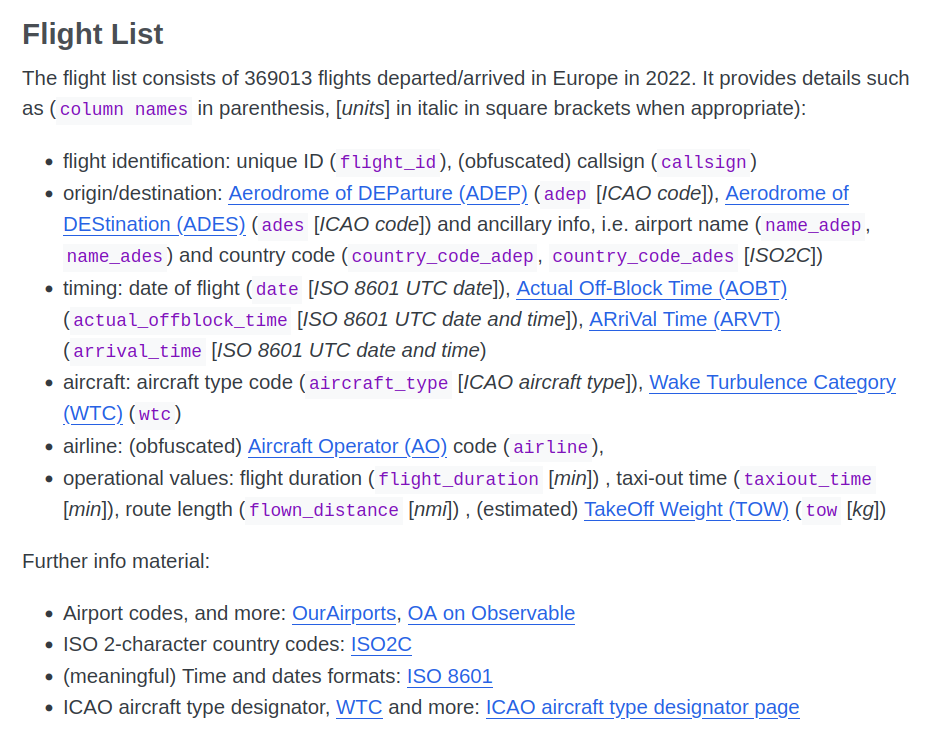
Dataset Details
The master dataset for this challenge was tabular data on 369k flights in Europe in 2022. This dataset enumerated all of the key datapoints for a given flight, such as aircraft type, origin and destination airports, amount of time flown, and known takeoff weight.
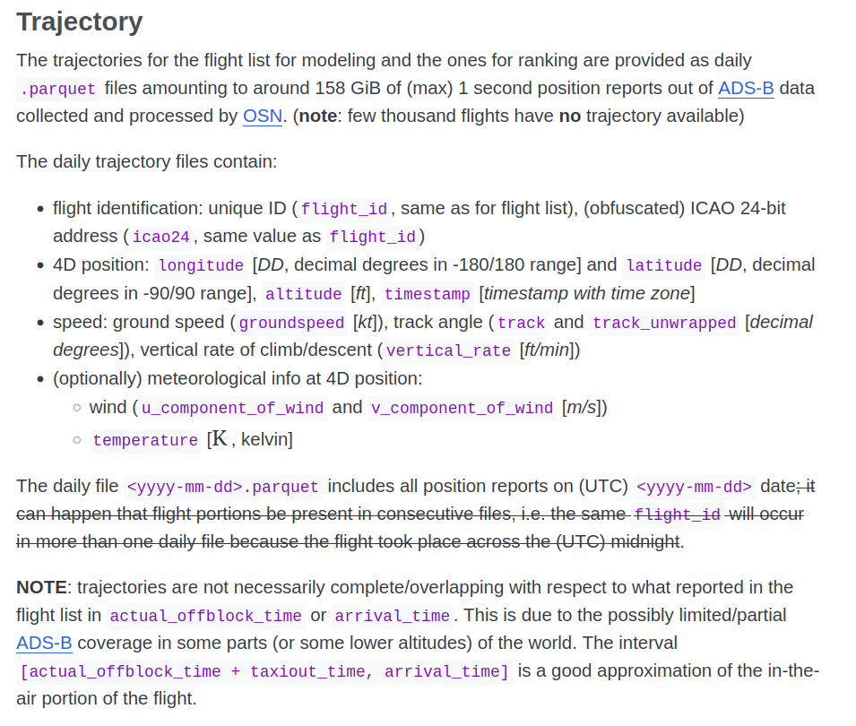
That dataset was supplemented with trajectory information from the OpenSky Network, captured every few seconds along the path of each flight, snapshotting essential information such as altitude, groundspeed, rate_of_climb, and current location.
Logging that data every couple seconds for each of the 369k flights in the dataset created a colossal amount of data - when all was said and done, the provided trajectories ended up taking up 306.4 GB on my hard drive in the form of daily Parquet files!
That volume was no joke and meant that it wouldn’t be possible to just “import” the trajectory data into some model and get any insights - you’d crash the computer instantly. Instead, I’d need to figure out what information I would want to extract from the trajectories, and then work to process the files down into a smaller, more wieldy dataset.
Processing the Trajectory Data

I performed all the compute for this project using my personal computer, a tiny Linux box tucked under my computer monitor. While peppy enough to make a few charts for my blog, it’s not exactly what you’d order to work on a “big data” project like this!
As such, the 306 GB of trajectory data was definitely daunting… but necessity is the mother of invention, and after some tinkering, I developed a working pipeline to process the trajectory data! The job took many hours to run (best done overnight, to be honest with you), but eventually distilled all that trajectory information down into a much more manageable 1.1GB dataset that I could then pull into my model.
Workflow
Since the trajectory data was stored in daily parquet files, I built my processing jobs to process a single day of data at a time, creating metrics at the flight_id level and outputting a new csv file with the output. That logic was contained inside my batch_process_trajectories.R file.
Some of the flight_id level features generated in the stage:
- time spent in different buckets of
vertical_rate, capturing seconds spent in climb, descent, and level flight - summary statistics like
mean,iqr,min, andmaxforaltitudeandgroundspeed - the
great_circle_distanceflown - time spent in different phases of wind, capturing time spent flying with
headwindsortailwinds
A simple Bash script called check_and_process.sh orchestrated all the job runs - it would loop over all of the files in the directory of parquet trajectory files, and if there was not already a csv output for that date, it would trigger a run of the job. Each run took about two minutes - times 365 days leaves us with twelve hours of continuous processing to crunch all these files. Poor tiny computer! Of course, I could have spun up a large EC2 instance and brute-forced the solution much faster, but the scrappy underdog in me had fun figuring out how to process the information I needed within the bounds of what was possible on my hardware.
Finally, I had a small R script called combine_trajectories.R to stitch all of the small daily csv files together into a single large (but not too large!) csv suitable for use in my model.
Workflow Files
batch_process_trajectories.R: read in a single .parquet trajectory file and output a .csv at the flight_id level with summarized detailscheck_and_process.sh: Bash script which checks to see all the .parquet files which have yet to be processed (ie. have a .csv output in the directory) and triggers the runs on outstanding filescombined_trajectories.Rmd: knits together the directory of daily .csvs into a single dataframe
Exploring the Base Data
With the trajectory data processed and ready to use later, I was excited to start exploring the primary dataset!
Anytime someone tosses me a new dataset with instructions to go build a predictive model, I need to do a few rounds of exploration to get a better sense of what I’m dealing with. As a visual learner, I find that getting summary statistics and then charting visualizations of the data is the quickest way to grasp how the data is laid out and what dimensions jump out.
In this case, I built a bunch of quick-and-dirty graphics which sought to explore how tow varied as a function of different variables. This helped give an immediate sense as to:
- the volume and variance of
towas a function of different dimensions, such asaircraft_type - the relationship between
towandflown_distancewhen normalized byaircraft_type - how the
towandflown_distancerelationship sees notable clustering effects when also sliced byairline
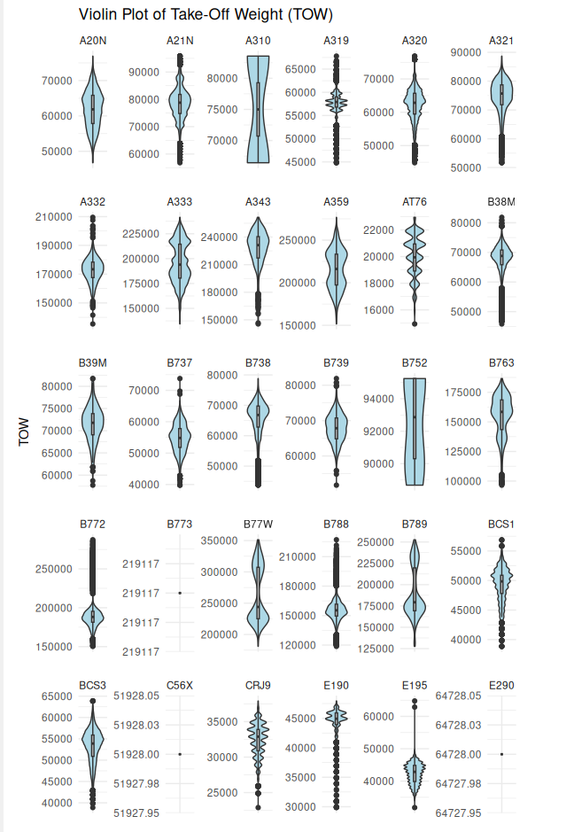
Violin Plot of TOW by Aircraft Type
This plot confirmed that there were a lot of distinct aircraft types in the data and also a meaningful amount of variance in the TOWs for each aircraft type.
ggplot(challenge_set, aes(x = "", y = tow)) +
  geom_violin(fill = "lightblue") +
  geom_boxplot(width = 0.1, fill = "grey") +
  facet_wrap(~aircraft_type, scales = "free") +
  labs(title = "Violin Plot of Take-Off Weight (TOW)", y = "TOW") +
  theme_minimal()
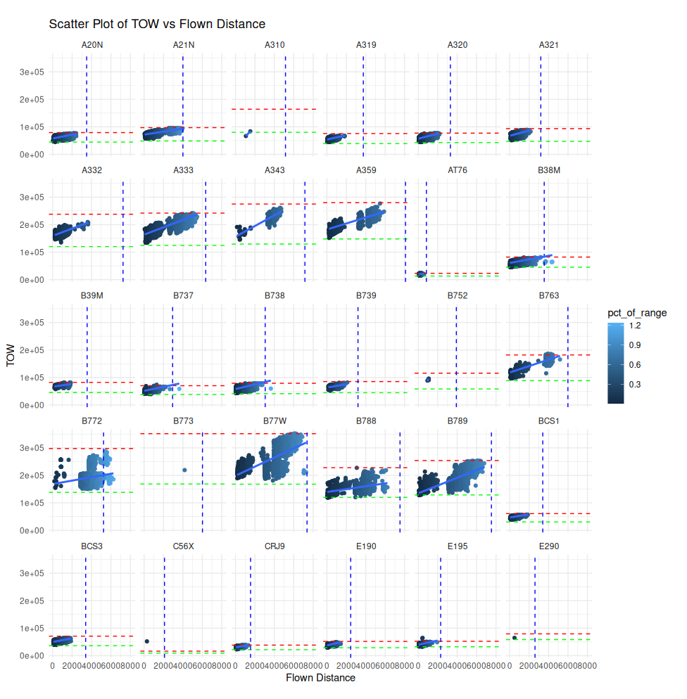
Scatterplot of TOW vs Flown Distance by Aircraft Type
TOW generally scaled upwards as a function of distance flown - no surprise there - but had very different slopes depending on the aircraft type in question.
ggplot(challenge_set, aes(x = flown_distance, y = tow, color = pct_of_range)) +
  geom_point() +
  facet_wrap(~ aircraft_type) +
  labs(title = "Scatter Plot of TOW vs Flown Distance", x = "Flown Distance", y = "TOW") +
  theme_minimal() +
  geom_hline(aes(yintercept = mtow), linetype = "dashed", color = "red") +
  geom_hline(aes(yintercept = oew), linetype = "dashed", color = "green") +
  geom_vline(aes(xintercept = range), linetype = "dashed", color = "blue") +
  geom_smooth(method = "lm")
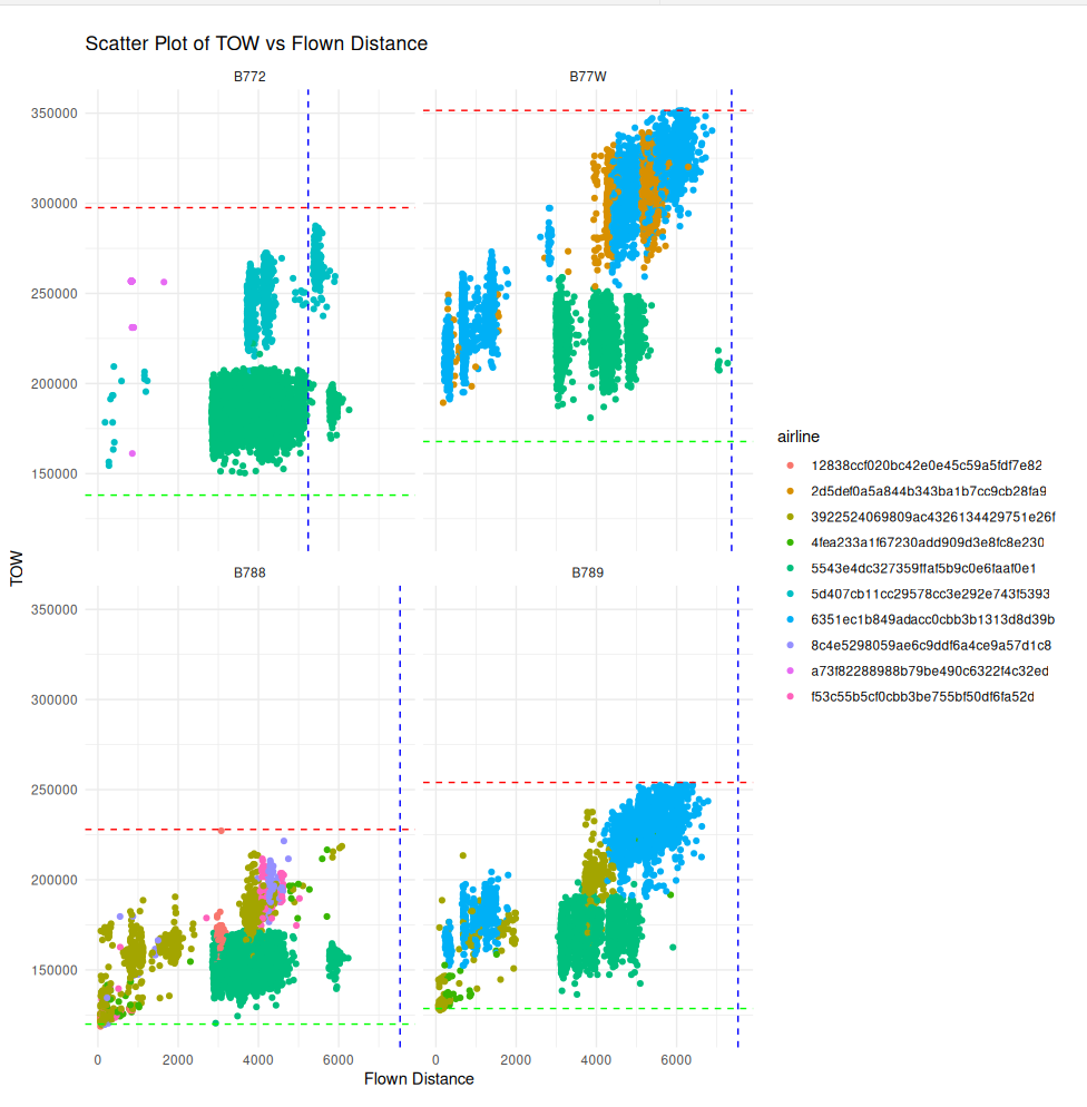
Scatterplot of TOW vs Flown Distance by Aircraft Type and Airline
Looking the TOW vs Flown Distance relationship for four notable widebody models (B772, B77W, B788, and B789) shows there is also a meaningful difference in usage between different airlines.
challenge_set %>%
  filter(aircraft_type %in% c("B772", "B77W", "B788", "B789")) %>%
  ggplot(aes(x = flown_distance, y = tow, color = airline)) +
    geom_point() +
    facet_wrap(~ aircraft_type) +
    labs(title = "Scatter Plot of TOW vs Flown Distance", x = "Flown Distance", y = "TOW") +
    theme_minimal() +
    geom_hline(aes(yintercept = mtow), linetype = "dashed", color = "red") +
    geom_hline(aes(yintercept = oew), linetype = "dashed", color = "green") +
    geom_vline(aes(xintercept = range), linetype = "dashed", color = "blue")
Building a Predictive Model
With the trajectory data processed into usable form and a few peeks taken at the data, I was finally ready to start building models!
Model Selection
Early on, I decided I would use a random forest to handle this regression task (estimating tow) - for a few reasons:
- Random forests aren’t black boxes: you can extract feature importance to learn about what features are particularly influential in your predictions
- Random forests handle a mix of categorical and continuous features with ease: they will naturally pick up on the distinct categories of
airlinein the data, without having to create dummy variables - Random forests are good at capturing nonlinear relationships between features: I thought we might see some on the margins of airplane range, flown distance, and
tow, so I wanted something which would find that signal rather than obscure it - Random forests are hard to overfit: because they are an ensemble of decision trees, where a random set of features is in use at each step, preventing any one pattern from dominating the model
Random forests aren’t perfect though - key drawbacks are:
- Random forests are slow to compute with large feature sets, since the complexity of the underlying decision trees scales upwards with the number of features
- Random forests don’t output coefficients nor do they unpack multicollinear effects: meaning that while the feature importances are helpful, they don’t show where the root causal effects might actually emerge, and correlated variables can increase total model accuracy, but distort the relative contributions of similar features
I did play with XGBoost for a second as an alternative to random forests, but didn’t get meaningfully better performance and so stuck with the random forest approach.
One note on implementation is that I had significant memory utilization issues by using the default implementation of randomForest in R - my model would continually max out the 16 GB of RAM on my computer and crash when being trained.
I was able to work around this by using ranger, an alternative implementation in R, which I was able to tune to use more CPU threads and less memory - making it feasible to do the model training on my tiny desktop.
Feature Engineering
In my experience, model selection (and tuning) is important, but choosing the right features to put into your model is even more important! A neural net or decision tree or even linear regression model is going to be pretty accurate if you are able to segment and summarize your data with strong features - but even the most robust models will fail to pick up on patterns if you haven’t done the work to carve out valuable features!
There were obviously a bunch of valuable features included right off the bat in the provided data: things like aircraft_type, flown_distance, and departure_airport - I piped those features straight into the model.
To get more accuracy I knew I would need to transform those features in a variety of ways, to try to “soak up” all the information they possessed about tow…
Here’s a list of what I ended up trying!
- Domain-specific Transformations: I generated new fields like
flown_velocityfrom the existingflown_distanceand departure/arrival times so the model could interpret the concept of “speed” in conjunction with the total flight time and distance - Continuous Variable Transformations: For most continuous features, I created log-transformations to reduce the skewness of the features. As needed, I also squared the features and took the square root of the features, so that non-linear relationships could emerge (ie. what if
flown_distancefor a particularaircraft_typestarts having a significant effect ontowas it approaches its maximum range?) - Categorizing and Bucketing: I grouped continuous features into categorical bins, like converting
departure_timeinto categories like'morning', 'afternoon', 'evening', or segmentingflown_distanceintoshort-haul, medium-haul, and long-haulflights. This helped capture hidden patterns in discrete segments of the data - Feature Interactions: I created interaction terms like
aircraft_type * departure_airportandflown_velocity * temperatureto capture how combinations of features impacttow. These interactions often surfaced hidden relationships that individual features could not capture alone - Model Stacking: I performed a quick-and-dirty linear regression using just
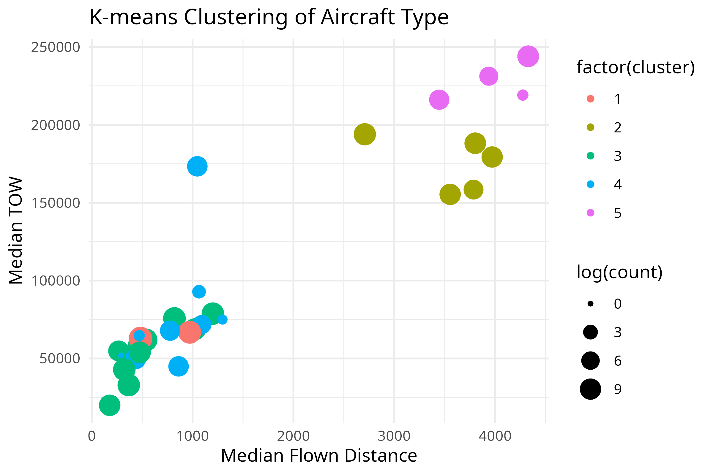
aircraft_modelandflown_distanceto predicttowfor eachflight_id, and then fed those predictions into my primary model as a new feature! This helped capture some small effects in the initial regression which the random forest could then build on - Dimensional Clustering: I used k-means clustering to develop a set of five clusters which grouped together similar
aircraft_types. This allowed the model to better general several distinct types of aircraft into a broader gestalt (ie. “large short-haul planes”, “medium long-haul planes”, “regional jets”) that could be used to analyze their collective behavior - Use of External Data: I pulled in publicly available data about airports to capture traits like their
elevation, and fetched information about eachaircraft_type’s maximum take-off weight (MTOW), original equipment weight (OEW), and range. This helped define the parameter space in which the model was making predictions - Collapsing Rare Categories: I found that the data had a few outlier
aircraft_typeandairlineswhich only had a handful of records. To not overfit the model to those rare categories, I instead collapsed them all down into a new “rare” category for the dimension in question, which helped the model be a bit more robust - Imputing Missing Data: For the handful of records which lacked trajectory data, or had values which didn’t make sense (ie. negative altitudes), I tried to “intelligently impute” what those values should have been, by looking at the other values observed for that flight or typical flights by that
aircraft_type
Model Training and Evaluation
Training the model was a pretty simple process - I took 80% of the fully featurized dataset used it to train the random forest, reserving the “unseen” 20% to make predictions on later, to measure the accuracy.
Accuracy was measured with a battery of metrics, but a primary focus on:
RMSE: root mean squared error - the target metric for the competition, this reflected “how off” my residuals were from the correcttowin units ofkilogramsMAPE: mean absolute percent error - a supplemental metric, this gave me a sense of what percent error I was seeing on average, a metrics that’s easier to compare when the data is sliced by different dimensions thanRMSE
Slice Data into Train and Test Sets
# Remove submission set rows from challenge_set
challenge_set <- challenge_set %>% filter(!is.na(tow))

# Test and Train split
sample_index <- sample(1:nrow(challenge_set), 0.8 * nrow(challenge_set))
train_data <- challenge_set[sample_index, ]
test_data <- challenge_set[-sample_index, ]
Train Random Forest
# Train random forest regression model
rf_model <- ranger(
  formula,
  data = train_data,
  importance = 'impurity',
  num.trees = 500,
  min.node.size = 5,
  save.memory = TRUE,
  replace = TRUE,
  sample.fraction = 0.7
)

# View the model summary
print(rf_model)
Evaluate Accuracy
# Make predictions on the test set
predictions <- predict(rf_model, data = test_data)$predictions

# Calculate MAPE
mape <- mean(abs((test_data$tow - predictions) / test_data$tow)) * 100
print(paste("MAPE: ", mape))

# Calculate RMSE
rmse <- sqrt(mse)
print(paste("Root Mean Squared Error: ", rmse))
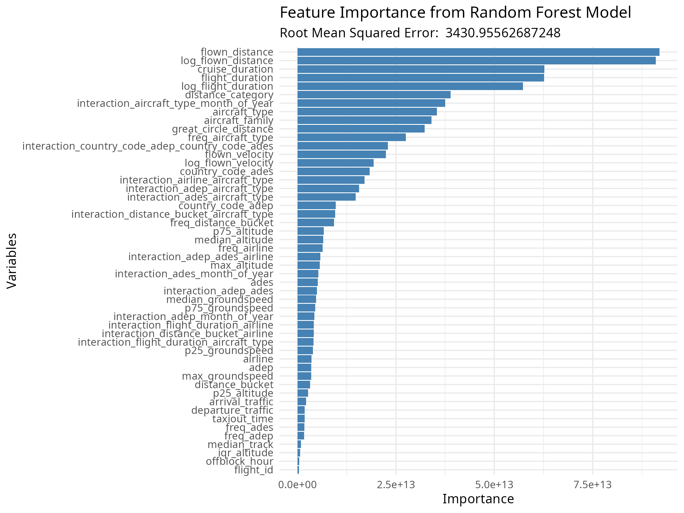
Understanding Feature Importance
Every time the model ran, it would 1) serialize itself to a file, and 2) generate an chart showing the relative importance of each feature in the model. Reviewing this each round of modeling allowed me to see which features seemed to be most useful, or not-useful at all - giving me a reason to tweak or expand on them in a future iteration of the model.
Here’s an early example, before I started interacting all the features and creating a bit of an explosion in total feature volume that makes the later charts very long to read:
# Grab the feature importances
importance_data <- as.data.frame(rf_model$variable.importance)

# Process the importance data
importance_data$Variable <- rownames(importance_data)
colnames(importance_data) <- c("Importance", "Variable")
importance_data <- importance_data[order(importance_data$Importance, decreasing = TRUE),]

# Build a barplot of importances
ggplot(importance_data, aes(x = reorder(Variable, Importance), y = Importance)) +
  geom_bar(stat = "identity", fill = "steelblue") +
  coord_flip() +
  xlab("Variables") +
  ylab("Importance") +
  ggtitle("Feature Importance from Random Forest Model") +
  labs(subtitle = paste("Root Mean Squared Error: ", rmse)) +
  theme_minimal()

# Export an image
ggsave(paste("training_results_", Sys.time(), ".png", sep = ""), path = "importances", height = 25, width = 8, units = "in", dpi = 300, bg = "white")
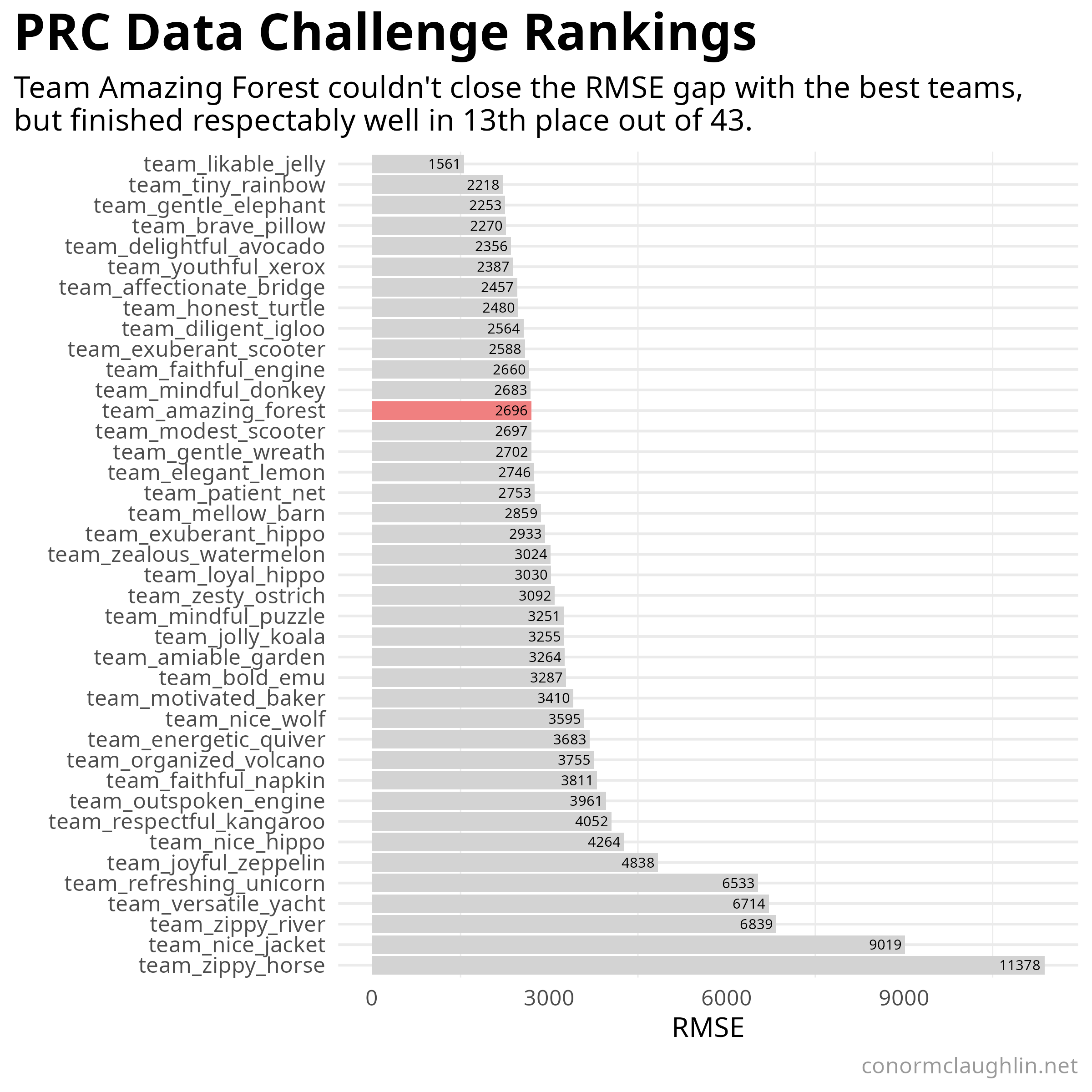
Challenge Results
Despite my best efforts and several weeks of iterative model tuning and feature engineering, I was never able to break into the “elite” tier of models submitted in the challenge! Ultimately, I finished in 13th place with a very respectable RMSE of 2,695 and a MAPE of less than 3% - solid figures, but a tier behind the silver and bronze finishers at roughly RMSE of roughly 2,250 and the winner with a borderline shocking RMSE of 1,561.
I am planning on writing a follow-up post to this one where I break down some of the approaches that the winning teams used in their code - things I might have missed or could have optimized better. Stay tuned for that follow-up post in a few days, and I hope that in the meantime you enjoyed this walkthrough of my model!
Fun Takeaways
- It took me 18 submissions to whittle my model RMSE down from about 3,500 to 2,600
- The final random forest model ended up having 302 independent features!
interaction_aircraft_family_distance_categorywas pretty stable as the most important feature for most of the time training- At the end, after implementing stacking, the
lm_predicted_tow_squaredfeature, sourced from the linear regression of the data, was the single most important feature logfeatures were typically more important than the original numbers- The A319 was the
aircraft_typeI was able to predict most accurately, with MAPE of 0.50%. The AT76 was the least accurate with MAPE of 3.38% - The B77W was the heaviest
aircraft_typein the data with averagetowof 264k kilograms, with the AT76 lowest at 20k MAPEgenerally went down as a function offlown_distance-towpredictions tended to be slightly less accurate on shorter flights- I was surprised that time features were not very useful at all - I expected features like month of year would have been very important, as they capture some amount of information about passenger loads and seasonal weather, but none of the month/week/day/time features I engineered seemed particularly important to the model
Code Reference
Process Trajectories
check_and_process.sh
#!/bin/bash

# Define directories
TRAJECTORIES_DIR="/home/conor/atow_predictions/trajectories"
PROCESSED_DIR="/home/conor/atow_predictions/processed_trajectories_v5"
R_SCRIPT_PATH="/home/conor/atow_predictions/batch_process_trajectories.R"

# Function to calculate the day of the year from YYYY-MM-DD
get_day_of_year() {
  date -d "$1" +%j
}

# Loop through all .parquet files in the trajectories directory
for parquet_file in "$TRAJECTORIES_DIR"/*.parquet
do
  # Extract the base filename (without extension)
  filename=$(basename -- "$parquet_file" .parquet)

  # Full path to the expected CSV file
  expected_csv="$PROCESSED_DIR/$filename.csv"

  # Print the filenames being checked for debugging
  echo "Checking if $expected_csv exists..."

  # Check if the corresponding .csv file exists in the processed directory
  if [ ! -f "$expected_csv" ]; then
    echo "$filename.csv is missing, processing $filename.parquet"

    # Calculate the day of the year from the filename (assumes format YYYY-MM-DD)
    day_of_year=$(get_day_of_year "$filename")

    # Run the R script with the day of the year as the parameter
    Rscript "$R_SCRIPT_PATH" "$day_of_year"
  else
    echo "$filename.csv already exists, skipping"
  fi
done
batch_process_trajectories.R
library(arrow)
library(tidyverse)
library(dplyr)
library(tidyr)
library(readr)
library(purrr)
library(e1071)


# Haversine formula function
haversine_distance <- function(lat1, lon1, lat2, lon2) {
  # Convert degrees to radians
  lat1 <- lat1 * pi / 180
  lon1 <- lon1 * pi / 180
  lat2 <- lat2 * pi / 180
  lon2 <- lon2 * pi / 180

  # Haversine formula
  dlat <- lat2 - lat1
  dlon <- lon2 - lon1
  a <- sin(dlat / 2)^2 + cos(lat1) * cos(lat2) * sin(dlon / 2)^2
  c <- 2 * atan2(sqrt(a), sqrt(1 - a))
  r <- 6371  # Radius of Earth in kilometers
  distance <- r * c

  return(distance)  # Return distance in KM
}

# https://sgichuki.github.io/Atmo/
windDir <-function(u,v){
  (270-atan2(u,v)*180/pi)%%360
}

windSpd <-function(u,v){
  sqrt(u^2+v^2)
}

# Function to process each file
process_file <- function(file_path) {
  # Open the dataset
  trajectory_df <- open_dataset(file_path)

  # Select only necessary columns to reduce memory load
  selected_data <- trajectory_df %>%
    select(flight_id, timestamp, groundspeed, altitude, latitude, longitude, vertical_rate, u_component_of_wind, v_component_of_wind, track, specific_humidity) %>%
    collect()  # Pull the data into R memory

  # Define speed and altitude bins after collecting
  vertical_rate_bins <- c(-Inf, -2000, -1000, -300, 300, 1000, 2000, Inf)  # Define bins for descent, level, and climb stages

  # Process and summarize the data in R
  time_spent_data <- selected_data %>%
    arrange(timestamp) %>%
    group_by(flight_id) %>%
    mutate(
      climb_stage = cut(vertical_rate, breaks = vertical_rate_bins, labels = FALSE),
      time_diff = as.numeric(difftime(lead(timestamp), timestamp, units = "secs"))
    ) %>%
    filter(!is.na(time_diff)) %>%
    group_by(flight_id, climb_stage) %>%
    summarise(total_time = sum(time_diff, na.rm = TRUE)) %>%
    ungroup()

  # Calculate total time for each flight
  total_time_per_flight <- time_spent_data %>%
    group_by(flight_id) %>%
    summarise(total_time_flight = sum(total_time, na.rm = TRUE))

  # Merge the total time back into the original dataset
  climb_time_spent <- time_spent_data %>%
    left_join(total_time_per_flight, by = "flight_id") %>%
    mutate(percentage_time = (total_time / total_time_flight) * 100)

  # Pivot to get time spent in each speed-altitude-climb category as columns
  time_spent_wide <- climb_time_spent %>%
    mutate(climb_category = paste0("climb_", climb_stage)) %>%
    select(flight_id, climb_category, total_time, percentage_time) %>%
    pivot_wider(
      names_from = climb_category,
      values_from = c(total_time, percentage_time),
      values_fill = 0
    )

  # Create a numeric timestamp variable
  selected_data$timestamp_numeric <- as.numeric(as.POSIXct(selected_data$timestamp))

  # Calculate wind speed and direction
  selected_data$wind_speed <- sqrt(selected_data$u_component_of_wind^2 + selected_data$v_component_of_wind^2)
  selected_data$wind_direction <- atan2(selected_data$v_component_of_wind, selected_data$u_component_of_wind) * (180 / pi)
  selected_data$wind_direction <- ifelse(selected_data$wind_direction < 0, selected_data$wind_direction + 360, selected_data$wind_direction)
  # Calculate relative wind angle (track vs wind)
  selected_data$relative_wind_angle <- (selected_data$track - selected_data$wind_direction + 180) %% 360 - 180
  # Calculate headwind/tailwind
  selected_data$headwind_tailwind <- selected_data$wind_speed * cos(selected_data$relative_wind_angle * (pi / 180))

  # Additional summary metrics per flight_id
  additional_metrics <- selected_data %>%
    group_by(flight_id) %>%
    summarise(
      count_trajectory_observations = n(),
      # Distance
      great_circle_distance = haversine_distance(first(latitude), first(longitude), last(latitude), last(longitude)),
      median_track = median(track, na.rm = TRUE),
      # Altitude
      max_altitude = quantile(altitude, probs = 0.99, na.rm = TRUE),
      median_altitude = median(altitude, na.rm = TRUE),
      p25_altitude = quantile(altitude, probs = 0.25, na.rm = TRUE),
      p75_altitude = quantile(altitude, probs = 0.75, na.rm = TRUE),
      iqr_altitude = IQR(altitude, na.rm = TRUE),
      sd_altitude = sd(altitude, na.rm = TRUE),
      # Groundspeed
      max_groundspeed = quantile(groundspeed, probs = 0.99, na.rm = TRUE),
      median_groundspeed = median(groundspeed, na.rm = TRUE),
      p25_groundspeed = quantile(groundspeed, probs = 0.25, na.rm = TRUE),
      p75_groundspeed = quantile(groundspeed, probs = 0.75, na.rm = TRUE),
      iqr_groundspeed = IQR(groundspeed, na.rm = TRUE),
      sd_groundspeed = sd(groundspeed, na.rm = TRUE),
      # Wind
      avg_headwind_tailwind = mean(headwind_tailwind, na.rm = TRUE),
      # Ascent Features
      max_vertical_rate = max(vertical_rate[vertical_rate > 0], na.rm = TRUE),   # Maximum climb rate
      avg_positive_vertical_rate = mean(vertical_rate[vertical_rate > 0], na.rm = TRUE),  # Average climb rate
      total_time_ascent = sum(diff(timestamp[vertical_rate > 300]), na.rm = TRUE), # Total time in ascent
      cumulative_ascent = sum(vertical_rate[vertical_rate > 300] * diff(timestamp_numeric[vertical_rate > 300]), na.rm = TRUE),
      # Descent Features
      min_vertical_rate = max(vertical_rate[vertical_rate < 0], na.rm = TRUE),   # Maximum descent rate
      avg_negative_vertical_rate = mean(vertical_rate[vertical_rate < 0], na.rm = TRUE),  # Average descent rate
      total_time_descent = sum(diff(timestamp[vertical_rate < 300]), na.rm = TRUE), # Total time in ascent
      cumulative_descent = sum(vertical_rate[vertical_rate < 300] * diff(timestamp_numeric[vertical_rate < 300]), na.rm = TRUE),
      # other
      avg_humidity = mean(specific_humidity, na.rm = TRUE),
      # Skew
      altitude_skewness = skewness(altitude, na.rm = TRUE),
      altitude_kurtosis = kurtosis(altitude, na.rm = TRUE),
      groundspeed_skewness = skewness(groundspeed, na.rm = TRUE),
      groundspeed_kurtosis = kurtosis(groundspeed, na.rm = TRUE)
    )

  # Define flight phases by altitude change and vertical rate
  selected_data <- selected_data %>%
    mutate(
      phase = case_when(
        altitude < 10000 & vertical_rate > 300 ~ "climb",
        altitude > 10000 & vertical_rate < 300 & vertical_rate > -300 ~ "cruise",
        altitude < 10000 & vertical_rate < -300 ~ "descent",
        TRUE ~ "other"
      )
    )

  # Summarise statistics for each phase
  phase_summary <- selected_data %>%
    group_by(flight_id, phase) %>%
    summarise(
      avg_altitude = mean(altitude, na.rm = TRUE),
      avg_groundspeed = mean(groundspeed, na.rm = TRUE),
      total_time_phase = sum(as.numeric(difftime(lead(timestamp), timestamp, units = "secs")), na.rm = TRUE)
    ) %>%
    pivot_wider(
      names_from = phase,
      values_from = c(avg_altitude, avg_groundspeed, total_time_phase),
      values_fill = 0
    )

  # Calculate rate of change of groundspeed
  selected_data <- selected_data %>%
    arrange(timestamp) %>%
    group_by(flight_id) %>%
    mutate(
      speed_diff = lead(groundspeed) - groundspeed,
      time_diff = as.numeric(difftime(lead(timestamp), timestamp, units = "secs")),
      acceleration = speed_diff / time_diff
    )

  # Summarize max/min acceleration and deceleration
  acceleration_summary <- selected_data %>%
    group_by(flight_id) %>%
    summarise(
      max_acceleration = max(acceleration, na.rm = TRUE),
      min_acceleration = min(acceleration, na.rm = TRUE)
    )

  # Calculate altitude IQR for each phase
  altitude_iqr_per_phase <- selected_data %>%
    group_by(flight_id, phase) %>%
    summarise(altitude_iqr = IQR(altitude, na.rm = TRUE)) %>%
    pivot_wider(
      names_from = phase,
      values_from = altitude_iqr,
      values_fill = 0,
      names_prefix = "altitude_iqr_"
    )

  # Fit a spline for altitude vs time for each flight
  # Extract features from the spline (e.g., curvature, inflection points)
  # spline_features <- selected_data %>%
  #   group_by(flight_id) %>%
  #   do(spline_model = smooth.spline(.$timestamp_numeric, .$altitude, spar = 0.5)) %>%
  #   reframe(
  #     flight_id,
  #     curvature = sum(abs(diff(spline_model$y, differences = 2))),  # Approx curvature
  #     num_inflection_points = sum(diff(sign(diff(spline_model$y))) != 0)  # Inflection points
  #   )

  # # Apply Fourier Transform to altitude vs time
  # # Extract the dominant frequency component
  # fourier_features <- selected_data %>%
  #   group_by(flight_id) %>%
  #   summarise(
  #     fft_altitude = fft(altitude),
  #     fft_groundspeed = fft(groundspeed),
  #   ) %>%
  #   summarise(
  #     dominant_freq_altitude = which.max(Mod(fft_altitude)),
  #     dominant_freq_groundspeed = which.max(Mod(fft_groundspeed))
  #   ) %>%
  #   mutate(
  #     dominant_freq_altitude = coalesce(dominant_freq_altitude, 0),  # Replace NA with 0
  #     dominant_freq_groundspeed = coalesce(dominant_freq_groundspeed, 0)  # Replace NA with 0
  #   )

  # Define altitude and groundspeed bins
  altitude_bins <- c(0, 5000, 10000, 15000, 20000, 25000, 30000, 35000, 40000, Inf)
  groundspeed_bins <- c(0, 100, 200, 300, 400, 500, 600, 700, Inf)

  # Create histogram features for cruise phase
  histogram_features <- selected_data %>%
    filter(phase == "cruise") %>%
    group_by(flight_id) %>%
    summarise(
      altitude_hist = list(hist(altitude, breaks = altitude_bins, plot = FALSE)$counts),
      groundspeed_hist = list(hist(groundspeed, breaks = groundspeed_bins, plot = FALSE)$counts)
    ) %>%
    unnest_wider(altitude_hist, names_sep = "_alt_bin_") %>%
    unnest_wider(groundspeed_hist, names_sep = "_speed_bin_")

  # Calculate the rate of phase transitions
  phase_transitions <- selected_data %>%
    group_by(flight_id) %>%
    mutate(phase_shift = lag(phase) != phase) %>%
    summarise(total_phase_transitions = sum(phase_shift, na.rm = TRUE))


  # Early and late segment summaries
  segment_summary <- selected_data %>%
    group_by(flight_id) %>%
    filter(timestamp_numeric <= min(timestamp_numeric) + 600 | timestamp_numeric >= max(timestamp_numeric) - 600) %>%
    mutate(segment = if_else(timestamp_numeric <= min(timestamp_numeric) + 600, "departure", "arrival")) %>%
    group_by(flight_id, segment) %>%
    summarise(
      avg_vertical_rate_segment = mean(vertical_rate, na.rm = TRUE),
      avg_groundspeed_segment = mean(groundspeed, na.rm = TRUE),
      avg_altitude_segment = mean(altitude, na.rm = TRUE)
    ) %>%
    pivot_wider(names_from = segment, values_from = c(avg_vertical_rate_segment, avg_groundspeed_segment, avg_altitude_segment), values_fill = 0)

  # Headwind and crosswind for each flight phase
  wind_phase_summary <- selected_data %>%
    group_by(flight_id, phase) %>%
    summarise(
      avg_headwind = mean(headwind_tailwind, na.rm = TRUE),
      avg_crosswind = mean(wind_speed * sin(relative_wind_angle * (pi / 180)), na.rm = TRUE)
    ) %>%
    pivot_wider(names_from = phase, values_from = c(avg_headwind, avg_crosswind), values_fill = 0)

  # Power indicators during climb and descent
  power_indicators <- selected_data %>%
    filter(phase %in% c("climb", "descent")) %>%
    group_by(flight_id, phase) %>%
    summarise(
      avg_power_ratio = mean(vertical_rate / groundspeed, na.rm = TRUE)  # Vertical rate-to-groundspeed ratio
    ) %>%
    pivot_wider(names_from = phase, values_from = avg_power_ratio, values_fill = 0, names_prefix = "power_ratio_")

  # Effective climb length in terms of time and distance
  climb_length <- selected_data %>%
    filter(phase == "climb") %>%
    group_by(flight_id) %>%
    summarise(
      climb_duration = sum(as.numeric(difftime(lead(timestamp), timestamp, units = "secs")), na.rm = TRUE),
      climb_distance = sum(haversine_distance(latitude, longitude, lead(latitude), lead(longitude)), na.rm = TRUE)
    )

  # Merge all feature sets together into the final summary
  final_summary <- time_spent_wide %>%
    left_join(additional_metrics, by = "flight_id") %>%
    left_join(phase_summary, by = "flight_id") %>%
    left_join(acceleration_summary, by = "flight_id") %>%
    left_join(altitude_iqr_per_phase, by = "flight_id") %>%
    left_join(wind_phase_summary, by = "flight_id") %>%
    left_join(histogram_features, by = "flight_id") %>%
    #left_join(spline_features, by = "flight_id") %>%
    #left_join(fourier_features, by = "flight_id") %>%
    left_join(phase_transitions, by = "flight_id") %>%
    left_join(wind_phase_summary, by = "flight_id") %>%
    left_join(segment_summary, by = "flight_id") %>%
    left_join(power_indicators, by = "flight_id") %>%
    left_join(climb_length, by = "flight_id")

  # Create CSV file name based on parquet file name
  csv_file_name <- gsub("\\.parquet$", ".csv", basename(file_path))

  # Write final_summary to CSV
  write_csv(final_summary, file.path("processed_trajectories_v5", csv_file_name))

  # Cleanup
  rm(list = ls())
  gc()

}

# Capture command-line arguments
args <- commandArgs(trailingOnly = TRUE)

# Extract the first argument
start_index <- as.numeric(args[1])
end_index <- start_index# + 1

# Print the parameter (or use it in your script)
cat("start_index:", start_index, "\t", "end_index:", end_index)

# Get a list of files to process
file_list <- list.files(path = "trajectories/", pattern = "*.parquet", full.names = TRUE)

# Iterate over files
walk(file_list[start_index:end_index], process_file)
combine_trajectories.R
library(tidyverse)
library(lubridate)
library(readr)

# Define the path to the directory containing CSV files
csv_directory <- "processed_trajectories_v5/"
file_list <- list.files(path = csv_directory, pattern = "*.csv", full.names = TRUE)

# Function to read and clean each file
read_and_clean_file <- function(file) {
  data <- read_csv(file, col_types = cols(.default = "c"))  # Read all columns as characters
  # Perform type conversion for specific columns
  data <- data %>%
    mutate(
      across(everything(), as.numeric),  # Try to convert all columns to numeric
      .names = "clean_{col}"
    ) %>%
    mutate(across(where(is.character), as.character))  # Convert remaining columns back to character if needed
  return(data)
}

# Apply the function to each file and combine results
combined_df <- file_list %>%
  lapply(read_and_clean_file) %>%
  bind_rows()  # Combine all data into a single DataFrame

write_csv(combined_df, "combined_trajectories_v5.csv")
Feature Engineering
Aircraft Type Clustering
For the first time:
aircraft_type_summary <- challenge_set %>%
  group_by(aircraft_type) %>%
  summarize(
    count = n(),
    distinct_operators = n_distinct(airline),
    median_flown_distance = median(flown_distance),
    min_flown_distance = min(flown_distance),
    max_flown_distance = max(flown_distance),
    median_flown_velocity = median(flight_duration) / median(flown_distance),
    max_flown_velocity = max(flight_duration / flown_distance),
    median_tow = median(tow, na.rm = TRUE),
    p25_tow = quantile(tow, 0.25, na.rm = TRUE)
  )

# do kmeans
set.seed(123)
kmeans_result <- aircraft_type_summary %>%
  select(count, distinct_operators, median_flown_distance, median_flown_velocity, median_tow) %>%
  scale() %>%
  kmeans(centers = 5)

# Add the cluster labels to the summarized data
aircraft_type_summary$cluster = kmeans_result$cluster

# Write to file for use later
aircraft_type_summary %>%
  select("aircraft_type", "cluster", "median_tow", "median_flown_distance", "count") %>%
  arrange(cluster) %>%
  write_csv("aircraft_type_clusters_kmeans.csv")

# Plot clusters
ggplot(aircraft_type_summary, aes(x = median_flown_distance, y = median_tow, size = log(count), color = factor(cluster))) +
  geom_point() +
  theme_minimal() +
  labs(
    title = "K-means Clustering of Aircraft Type",
    x = "Median Flown Distance",
    y = "Median TOW"
  )
On future runs:
aircraft_type_clusters_kmeans <- read_csv("aircraft_type_clusters_kmeans.csv") %>%
  select("aircraft_type", "cluster") %>%
  rename("aircraft_type_cluster" = "cluster")

aircraft_type_clusters_kmeans$aircraft_type_cluster = as.factor(aircraft_type_clusters_kmeans$aircraft_type_cluster)

challenge_set <- merge(x = challenge_set, y = aircraft_type_clusters_kmeans, by = "aircraft_type", all.x = TRUE)
Linear Regression
# Fit linear regression models by aircraft_type and get predicted values
challenge_set <- challenge_set %>%
  group_by(aircraft_type) %>%
  do({
    model <- lm(tow ~ flown_distance, data = na.omit(.))
    data.frame(., lm_predicted_tow = predict(model, newdata = .))
  }) %>%
  ungroup()

# Fit linear regression models by aircraft_type and extract R²
r_squared_values <- challenge_set %>%
  group_by(aircraft_type) %>%
  do(model = lm(tow ~ flown_distance, data = na.omit(.))) %>%
  summarise(aircraft_type,
            lm_predicted_tow_r_squared = summary(model)$r.squared
            )

challenge_set <- merge(x = challenge_set, y = r_squared_values, by = "aircraft_type", all.x = TRUE)
Feature Transformations
# Loop over each column and collapse rare categories
for (column in columns_to_collapse_prop) {
  challenge_set <- collapse_rare_categories_by_prop(challenge_set, column, prop_threshold = 0.0025, new_category = "Rare")
}

columns_to_collapse_abs <- c("adep", "ades", "country_code_ades", "country_code_adep")

# Loop over each column and collapse rare categories
for (column in columns_to_collapse_abs) {
  challenge_set <- collapse_rare_categories_by_count(challenge_set, column, min_count = 3, new_category = "Rare")
}
challenge_set <- challenge_set %>%
  mutate(
    offblock_time_of_day = case_when(
      hour(actual_offblock_time) %in% c(6,7,8,9,10,11) ~ 'Morning',
      hour(actual_offblock_time) %in% c(12,13,14,15,16,17) ~ 'Afternoon',
      hour(actual_offblock_time) %in% c(18,19,20,21,22,23) ~ 'Evening',
      hour(actual_offblock_time) %in% c(0,1,2,3,4,5) ~ 'Night',
      .default = 'Unknown'
    ),
    offblock_is_peak = case_when(
      hour(actual_offblock_time) %in% c(7,8,17,18) ~ 'Peak',
      .default = 'Off Peak'
    ),
    arrival_time_of_day = case_when(
      hour(arrival_time) %in% c(6,7,8,9,10,11) ~ 'Morning',
      hour(arrival_time) %in% c(12,13,14,15,16,17) ~ 'Afternoon',
      hour(arrival_time) %in% c(18,19,20,21,22,23) ~ 'Evening',
      hour(arrival_time) %in% c(0,1,2,3,4,5) ~ 'Night',
      .default = 'Unknown'
    ),
    arrival_is_peak = case_when(
      hour(arrival_time) %in% c(7,8,17,18) ~ 'Peak',
      .default = 'Off Peak'
    ),
    day_of_week = wday(date, label = TRUE),
    is_weekend = if_else(wday(date, label = TRUE) %in% c('Sat', 'Sun'), TRUE, FALSE),
    week_of_year = as.factor(isoweek(date)),
    month_of_year = month(date, label = TRUE),
    is_domestic = if_else(country_code_adep == country_code_ades, TRUE, FALSE),
    flown_velocity = flown_distance / flight_duration,
    aircraft_family = substr(aircraft_type, 1, 3),
    distance_category = cut(flown_distance, breaks = c(0, 1000, 2700, Inf), labels = c("short", "medium", "long")),
    distance_bucket = coalesce(cut(flown_distance,
                          breaks = seq(0, quantile(flown_distance, 0.999, na.rm = TRUE) + 500, by = 500),
                          right = FALSE,
                          include.lowest = TRUE), 'other'),
    flown_velocity_bucket = cut(flown_distance / flight_duration, breaks = seq(0, max(flown_distance / flight_duration, na.rm = TRUE) + 1, by = 0.5), right = FALSE, include.lowest = TRUE),
    relative_distance_adep_ades = cut(flown_distance / ave(flown_distance, adep, ades, FUN = mean), breaks = 10),
    relative_distance_aircraft_type = flown_distance / ave(flown_distance, aircraft_type, FUN = mean),
    relative_flown_velocity_aircraft_type = (flown_distance / flight_duration) / ave((flown_distance / flight_duration), aircraft_type, FUN = mean),
    relative_distance_adep_ades_aircraft_type = cut(flown_distance / ave(flown_distance, adep, ades, aircraft_type, FUN = mean), breaks = 10),
    relative_distance_airline = flown_distance / ave(flown_distance, airline, FUN = mean),
    relative_distance_aircraft_type_airline = flown_distance / ave(flown_distance, aircraft_type, airline, FUN = mean),
    cruise_duration = pmax(flight_duration - 30, 0),
    flight_minus_taxiout_duration_bucket = coalesce(cut(pmax(flight_duration - taxiout_time, 0),
                                               breaks = seq(0, quantile(pmax(flight_duration - taxiout_time, 0), 0.999, na.rm = TRUE) + 30, by = 30),  # Adjust flight_minus_taxiout_duration_bucket based on 99.9th percentile
                                               right = FALSE,
                                               include.lowest = TRUE), 'other'),
    departure_traffic = ave(flight_id, adep, date, FUN = length),
    arrival_traffic = ave(flight_id, ades, date, FUN = length),
    departure_traffic_squared = departure_traffic ^ 2,
    arrival_traffic_squared = arrival_traffic ^ 2,
    departure_traffic_bucket = cut(departure_traffic, breaks = 10),
    arrival_traffic_bucket = cut(arrival_traffic, breaks = 10),
    product_departure_traffic_arrival_traffic = departure_traffic * arrival_traffic,
    log_flight_duration = log1p(flight_duration),
    log_flown_distance = log1p(flown_distance),
    log_flown_distance_bucket = cut(log1p(flown_distance), breaks = 10),
    log_flown_velocity = log1p(flown_distance / flight_duration),
    flown_distance_squared = flown_distance ^ 2,
    flown_distance_sqrt = sqrt(flown_distance),
    flown_velocity_squared = (flown_distance / flight_duration) ^ 2,
    flown_velocity_sqrt = sqrt(flown_distance / flight_duration),
    taxiout_time_bucket = cut(taxiout_time, breaks = 10),
    taxiout_time_squared = taxiout_time ^ 2,
    taxiout_to_flight_duration_ratio = taxiout_time / flight_duration,
    taxiout_to_flight_duration_sqrt = sqrt(taxiout_time / flight_duration),
    log_great_circle_distance_adep_ades = log1p(great_circle_distance_adep_ades),
    great_circle_distance_squared = great_circle_distance_adep_ades ^ 2,
    great_circle_distance_sqrt = sqrt(great_circle_distance_adep_ades),
    log_median_altitude = log1p(median_altitude),
    median_altitude_squared = median_altitude ^ 2,
    log_median_groundspeed = log1p(median_groundspeed),
    altitude_range = p75_altitude - p25_altitude,
    groundspeed_range = p75_groundspeed - p25_groundspeed,
    altitude_range_bucket = cut(altitude_range, breaks = 10),
    groundspeed_range_bucket = cut(groundspeed_range, breaks = 10),
    flown_distance_over_great_circle = flown_distance / great_circle_distance_adep_ades,
    great_circle_distance_bucket = coalesce(cut(great_circle_distance_adep_ades,
                                       breaks = seq(0, quantile(great_circle_distance_adep_ades, 0.999, na.rm = TRUE) + 500, by = 500),  # Adjust great_circle_distance_bucket based on 99.9th percentile
                                       right = FALSE,
                                       include.lowest = TRUE), 'other'),
    total_time_ascent_squared = total_time_ascent ^ 2,
    total_time_ascent_bucket = cut(total_time_ascent, breaks = 10),
    total_time_descent_squared = total_time_descent ^ 2,
    total_time_descent_bucket = cut(total_time_descent, breaks = 10),
    pct_total_time_ascent = total_time_ascent / flight_duration,
    pct_total_time_descent = total_time_descent / flight_duration,
    mtow_oew_diff = mtow - oew,
    pct_max_flown_distance_by_aircraft_type = cut((flown_distance / ave(flown_distance, aircraft_type, FUN = max)), breaks = 10),
    headwind_tailwind_bucket = cut(avg_headwind_tailwind, breaks = 10),
    avg_humidity_sqrt = sqrt(avg_humidity),
    avg_humidity_bucket = cut(avg_humidity_sqrt, breaks = 10),
    flown_distance_pct_range = flown_distance / range,
    predicted_tow_category = cut(lm_predicted_tow, breaks = quantile(lm_predicted_tow, probs = seq(0, 1, 0.1)), include.lowest = TRUE),
    lm_predicted_tow_squared = lm_predicted_tow^2,
    lm_predicted_tow_cubed = lm_predicted_tow^3,
    log_lm_predicted_tow = log(lm_predicted_tow + 1),
    r_squared_category = cut(lm_predicted_tow_r_squared,
                                         breaks = c(-Inf, 0, 0.5, 0.7, 0.9, 1),
                                         labels = c("Very Poor", "Poor", "Average", "Good", "Excellent"),
                                         include.lowest = TRUE)

  )
Interaction Variables
# aircraft type cluster
challenge_set$interaction_aircraft_type_cluster_log_great_circle_distance_adep_ades <- interaction(challenge_set$aircraft_type_cluster, challenge_set$log_great_circle_distance_adep_ades)
challenge_set$interaction_aircraft_type_cluster_log_flown_distance <- interaction(challenge_set$aircraft_type_cluster, challenge_set$log_flown_distance)
challenge_set$interaction_aircraft_type_cluster_log_flight_duration <- interaction(challenge_set$aircraft_type_cluster, challenge_set$log_flight_duration)
challenge_set$interaction_aircraft_type_cluster_flown_distance_squared <- interaction(challenge_set$aircraft_type_cluster, challenge_set$flown_distance_squared)
challenge_set$interaction_aircraft_type_cluster_cruise_duration <- interaction(challenge_set$aircraft_type_cluster, challenge_set$cruise_duration)
challenge_set$interaction_aircraft_type_cluster_total_time_ascent <- interaction(challenge_set$aircraft_type_cluster, challenge_set$total_time_ascent)
challenge_set$interaction_aircraft_type_cluster_airline <- interaction(challenge_set$airline, challenge_set$aircraft_type_cluster)
challenge_set$interaction_aircraft_type_cluster_adep <- interaction(challenge_set$adep, challenge_set$aircraft_type_cluster)
challenge_set$interaction_aircraft_type_cluster_ades <- interaction(challenge_set$ades, challenge_set$aircraft_type_cluster)
challenge_set$interaction_aircraft_type_cluster_distance_bucket <- interaction(challenge_set$distance_bucket, challenge_set$aircraft_type_cluster)
challenge_set$interaction_aircraft_type_cluster_flown_velocity_bucket <- interaction(challenge_set$aircraft_type_cluster, challenge_set$flown_velocity_bucket)
challenge_set$interaction_aircraft_type_cluster_median_altitude <- interaction(challenge_set$aircraft_type_cluster, challenge_set$median_altitude)
challenge_set$interaction_aircraft_type_cluster_log_median_altitude <- interaction(challenge_set$aircraft_type_cluster, challenge_set$log_median_altitude)
challenge_set$interaction_aircraft_type_cluster_p25_altitude <- interaction(challenge_set$aircraft_type_cluster, challenge_set$p25_altitude)
challenge_set$interaction_aircraft_type_cluster_max_altitude <- interaction(challenge_set$aircraft_type_cluster, challenge_set$max_altitude)
challenge_set$interaction_aircraft_type_cluster_total_time_ascent <- interaction(challenge_set$total_time_ascent, challenge_set$aircraft_type_cluster)
challenge_set$interaction_aircraft_type_cluster_total_time_descent <- interaction(challenge_set$total_time_descent, challenge_set$aircraft_type_cluster)
challenge_set$interaction_aircraft_type_cluster_total_time_climb_4 <- interaction(challenge_set$total_time_climb_4, challenge_set$aircraft_type_cluster)
challenge_set$interaction_aircraft_type_cluster_percentage_time_climb_4 <- interaction(challenge_set$percentage_time_climb_4, challenge_set$aircraft_type_cluster)
challenge_set$interaction_aircraft_type_cluster_month_of_year <- interaction(challenge_set$aircraft_type_cluster, challenge_set$month_of_year)
challenge_set$interaction_aircraft_type_cluster_country_code_ades <- interaction(challenge_set$aircraft_type_cluster, challenge_set$country_code_ades)
challenge_set$interaction_aircraft_type_cluster_log_flown_velocity <- interaction(challenge_set$aircraft_type_cluster, challenge_set$log_flown_velocity)
challenge_set$interaction_aircraft_family_distance_category <- interaction(challenge_set$aircraft_family, challenge_set$distance_category)
challenge_set$interaction_aircraft_type_cluster_product_departure_traffic_arrival_traffic <- interaction(challenge_set$aircraft_type_cluster, challenge_set$product_departure_traffic_arrival_traffic)
challenge_set$interaction_aircraft_type_distance_bucket_airline <- interaction(challenge_set$distance_bucket, challenge_set$aircraft_type, challenge_set$aircraft_type)

# aircraft type
challenge_set$interaction_aircraft_type_distance_bucket <- interaction(challenge_set$distance_bucket, challenge_set$aircraft_type)
challenge_set$interaction_aircraft_type_flight_minus_taxiout_duration_bucket <- interaction(challenge_set$flight_minus_taxiout_duration_bucket, challenge_set$aircraft_type)
challenge_set$interaction_aircraft_type_flown_velocity_bucket <- interaction(challenge_set$aircraft_type, challenge_set$flown_velocity_bucket)
challenge_set$interaction_aircraft_type_median_altitude <- interaction(challenge_set$aircraft_type, challenge_set$median_altitude)
challenge_set$interaction_aircraft_type_offblock_time_of_day <- interaction(challenge_set$offblock_time_of_day, challenge_set$aircraft_type)
challenge_set$interaction_aircraft_type_month_of_year <- interaction(challenge_set$aircraft_type, challenge_set$month_of_year)
challenge_set$interaction_aircraft_type_offblock_is_peak <- interaction(challenge_set$aircraft_type, challenge_set$offblock_is_peak)
challenge_set$interaction_aircraft_type_pct_max_distance_flown_by_aircraft_type <- interaction(challenge_set$aircraft_type, challenge_set$pct_max_flown_distance_by_aircraft_type)
challenge_set$interaction_aircraft_type_altitude_range_bucket <- interaction(challenge_set$aircraft_type, challenge_set$altitude_range_bucket)
challenge_set$interaction_aircraft_type_groundspeed_range_bucket <- interaction(challenge_set$aircraft_type, challenge_set$groundspeed_range_bucket)
challenge_set$interaction_aircraft_type_elevation_ft_adep <- interaction(challenge_set$aircraft_type, challenge_set$elevation_ft_adep)
challenge_set$interaction_aircraft_type_country_code_adep <- interaction(challenge_set$aircraft_type, challenge_set$country_code_adep)
challenge_set$interaction_aircraft_type_country_code_ades <- interaction(challenge_set$aircraft_type, challenge_set$country_code_ades)
challenge_set$interaction_aircraft_type_airline <- interaction(challenge_set$aircraft_type, challenge_set$airline)
challenge_set$interaction_aircraft_type_adep <- interaction(challenge_set$aircraft_type, challenge_set$adep)
challenge_set$interaction_aircraft_type_ades <- interaction(challenge_set$aircraft_type, challenge_set$ades)
challenge_set$interaction_aircraft_type_aircraft_family <- interaction(challenge_set$aircraft_type, challenge_set$aircraft_family)
challenge_set$interaction_aircraft_type_taxiout_time_bucket <- interaction(challenge_set$aircraft_type, challenge_set$taxiout_time_bucket)
challenge_set$interaction_aircraft_type_month_of_year <- interaction(challenge_set$aircraft_type, challenge_set$month_of_year)
challenge_set$interaction_aircraft_type_offblock_time_of_day <- interaction(challenge_set$aircraft_type, challenge_set$offblock_time_of_day)
challenge_set$interaction_aircraft_type_offblock_is_peak <- interaction(challenge_set$aircraft_type, challenge_set$offblock_is_peak)
challenge_set$interaction_aircraft_type_total_time_ascent_bucket <- interaction(challenge_set$aircraft_type, challenge_set$total_time_ascent_bucket)
challenge_set$interaction_aircraft_type_total_time_descent_bucket <- interaction(challenge_set$aircraft_type, challenge_set$total_time_descent_bucket)
challenge_set$interaction_aircraft_type_departure_traffic_bucket <- interaction(challenge_set$aircraft_type, challenge_set$departure_traffic_bucket)
challenge_set$interaction_aircraft_type_distance_category <- interaction(challenge_set$aircraft_type, challenge_set$distance_category)
challenge_set$interaction_aircraft_type_product_departure_traffic_arrival_traffic <- interaction(challenge_set$aircraft_type, challenge_set$product_departure_traffic_arrival_traffic)
challenge_set$interaction_aircraft_type_predicted_tow <- interaction(challenge_set$aircraft_type, challenge_set$lm_predicted_tow)


# airline
interaction_airline_flight_duration <- interaction(challenge_set$airline, challenge_set$flight_duration)
interaction_airline_great_circle_distance <- interaction(challenge_set$airline, challenge_set$great_circle_distance_adep_ades)
interaction_airline_flown_distance <- interaction(challenge_set$airline, challenge_set$flown_distance)
challenge_set$interaction_airline_aircraft_type <- interaction(challenge_set$airline, challenge_set$aircraft_type)
challenge_set$interaction_airline_distance_bucket <- interaction(challenge_set$distance_bucket, challenge_set$airline)
challenge_set$interaction_airline_distance_category <- interaction(challenge_set$distance_category, challenge_set$airline)
challenge_set$interaction_airline_flight_minus_taxiout_duration_bucket <- interaction(challenge_set$flight_minus_taxiout_duration_bucket, challenge_set$airline)
challenge_set$interaction_airline_offblock_time_of_day <- interaction(challenge_set$distance_bucket, challenge_set$offblock_time_of_day)
challenge_set$interaction_airline_product_departure_traffic_arrival_traffic <- interaction(challenge_set$airline, challenge_set$product_departure_traffic_arrival_traffic)
interaction_airline_offblock_is_peak <- interaction(challenge_set$airline, challenge_set$offblock_is_peak)
interaction_airline_month_of_year <- interaction(challenge_set$airline, challenge_set$month_of_year)
interaction_airline_day_of_week <- interaction(challenge_set$airline, challenge_set$day_of_week)
interaction_airline_distance_category <- interaction(challenge_set$airline, challenge_set$distance_category)
interaction_airline_country_code_adep <- interaction(challenge_set$airline, challenge_set$country_code_adep)
interaction_airline_country_code_ades <- interaction(challenge_set$airline, challenge_set$country_code_ades)
interaction_airline_departure_traffic <- interaction(challenge_set$airline, challenge_set$departure_traffic)
interaction_airline_taxiout_time <- interaction(challenge_set$airline, challenge_set$taxiout_time)
interaction_airline_total_time_ascent <- interaction(challenge_set$airline, challenge_set$total_time_ascent)
interaction_airline_flight_minus_taxiout_duration_bucket <- interaction(challenge_set$airline, challenge_set$flight_minus_taxiout_duration_bucket)
interaction_airline_flown_velocity_bucket <- interaction(challenge_set$airline, challenge_set$flown_velocity_bucket)
interaction_airline_altitude_range_bucket <- interaction(challenge_set$airline, challenge_set$altitude_range_bucket)
interaction_airline_avg_humidity_bucket <- interaction(challenge_set$airline, challenge_set$avg_humidity_bucket)
interaction_airline_distance_bucket <- interaction(challenge_set$airline, challenge_set$distance_bucket)
interaction_airline_headwind_tailwind_bucket <- interaction(challenge_set$airline, challenge_set$headwind_tailwind_bucket)


# adep
challenge_set$interaction_adep_airline <- interaction(challenge_set$adep, challenge_set$airline)
challenge_set$interaction_adep_aircraft_type <- interaction(challenge_set$adep, challenge_set$aircraft_type)
challenge_set$interaction_adep_month_of_year <- interaction(challenge_set$adep, challenge_set$month_of_year)
challenge_set$interaction_adep_ades <- interaction(challenge_set$adep, challenge_set$ades)
challenge_set$interaction_adep_ades_airline <- interaction(challenge_set$interaction_adep_ades, challenge_set$airline)
challenge_set$interaction_adep_distance_bucket <- interaction(challenge_set$adep, challenge_set$distance_bucket)
challenge_set$interaction_adep_flown_distance_squared <- interaction(challenge_set$adep, challenge_set$flown_distance_squared)

# ades
challenge_set$interaction_ades_airline <- interaction(challenge_set$ades, challenge_set$airline)
challenge_set$interaction_ades_aircraft_type <- interaction(challenge_set$ades, challenge_set$aircraft_type)
challenge_set$interaction_ades_month_of_year <- interaction(challenge_set$ades, challenge_set$month_of_year)
challenge_set$interaction_country_code_ades_country_code_adep <- interaction(challenge_set$country_code_ades, challenge_set$country_code_adep)
challenge_set$interaction_country_code_ades_flown_distance_bucket <- interaction(challenge_set$country_code_ades, challenge_set$distance_bucket)
challenge_set$interaction_country_code_ades_flown_distance_squared <- interaction(challenge_set$country_code_ades, challenge_set$flown_distance_squared)

# time
challenge_set$interaction_day_of_week_departure_traffic <- interaction(challenge_set$day_of_week, challenge_set$departure_traffic)
challenge_set$interaction_month_of_year_aircraft_type_cluster_flown_distance_bucket <- interaction(challenge_set$month_of_year, challenge_set$aircraft_type_cluster, challenge_set$distance_bucket)
challenge_set$interaction_distance_bucket_offblock_time_of_day <- interaction(challenge_set$distance_bucket, challenge_set$offblock_time_of_day)

# great_circle_distance_bucket
challenge_set$interaction_great_circle_distance_bucket_aircraft_type_cluster <- interaction(challenge_set$great_circle_distance_bucket, challenge_set$aircraft_type_cluster)
challenge_set$interaction_great_circle_distance_bucket_aircraft_type <- interaction(challenge_set$great_circle_distance_bucket, challenge_set$aircraft_type)
challenge_set$interaction_great_circle_distance_bucket_flown_velocity_bucket <- interaction(challenge_set$great_circle_distance_bucket, challenge_set$flown_velocity_bucket)
challenge_set$interaction_great_circle_distance_bucket_country_code_ades <- interaction(challenge_set$great_circle_distance_bucket, challenge_set$country_code_ades)
challenge_set$interaction_great_circle_distance_bucket_median_altitude <- interaction(challenge_set$great_circle_distance_bucket, challenge_set$median_altitude)

# continuous variable interactions
challenge_set$interaction_log_great_circle_distance_adep_ades_log_median_altitude <- interaction(challenge_set$log_great_circle_distance_adep_ades, challenge_set$log_median_altitude)
challenge_set$interaction_distance_category_median_groundspeed <- interaction(challenge_set$distance_category, challenge_set$median_groundspeed)
challenge_set$interaction_total_time_ascent_aircraft_type <- interaction(challenge_set$total_time_ascent, challenge_set$aircraft_type)
challenge_set$interaction_total_time_descent_aircraft_type <- interaction(challenge_set$total_time_descent, challenge_set$aircraft_type)
challenge_set$interaction_altitude_range_bucket_distance_bucket <- interaction(challenge_set$altitude_range_bucket, challenge_set$distance_bucket)
challenge_set$interaction_groundspeed_range_distance_bucket <- interaction(challenge_set$groundspeed_range_bucket, challenge_set$distance_bucket)

# Catchall
challenge_set$interaction_taxiout_time_flown_distance <- interaction(challenge_set$taxiout_time, challenge_set$flown_distance)
challenge_set$interaction_taxiout_time_great_circle_distance_adep_ades <- interaction(challenge_set$taxiout_time, challenge_set$great_circle_distance_adep_ades)
challenge_set$interaction_log_flown_distance_offblock_time_of_day <- interaction(challenge_set$log_flown_distance, challenge_set$offblock_time_of_day)
challenge_set$interaction_total_time_ascent_offblock_is_peak <- interaction(challenge_set$total_time_ascent, challenge_set$offblock_is_peak)
challenge_set$interaction_month_of_year_log_flown_distance <- interaction(challenge_set$month_of_year, challenge_set$log_flown_distance)
challenge_set$interaction_headwind_tailwind_bucket_altitude_range_bucket <- interaction(challenge_set$headwind_tailwind_bucket, challenge_set$altitude_range_bucket)
challenge_set$interaction_avg_humidity_bucket_total_time_ascent_bucket <- interaction(challenge_set$avg_humidity_bucket, challenge_set$total_time_ascent_bucket)
challenge_set$interaction_oew_flown_distance <- interaction(challenge_set$oew, challenge_set$flown_distance)
challenge_set$interaction_mtw_oew_diff_distance_bucket <- interaction(challenge_set$mtow_oew_diff, challenge_set$distance_bucket)
challenge_set$interaction_country_code_adep_elevation_ft_adep <- interaction(challenge_set$country_code_adep, challenge_set$elevation_ft_adep)
challenge_set$interaction_country_code_ades_elevation_ft_ades <- interaction(challenge_set$country_code_ades, challenge_set$elevation_ft_ades)
challenge_set$interaction_departure_traffic_distance_category <- interaction(challenge_set$departure_traffic, challenge_set$distance_category)
challenge_set$interaction_log_flown_distance_bucket_altitude_range_bucket <- interaction(challenge_set$log_flown_distance_bucket, challenge_set$altitude_range_bucket)
challenge_set$interaction_offblock_time_of_day_log_flown_distance_bucket <- interaction(challenge_set$offblock_time_of_day, challenge_set$log_flown_distance_bucket)
challenge_set$interaction_flight_duration_day_of_week <- interaction(challenge_set$flight_duration, challenge_set$day_of_week)
challenge_set$interaction_flight_duration_is_weekend <- interaction(challenge_set$flight_duration, challenge_set$is_weekend)
challenge_set$interaction_offblock_is_peak_month_of_year <- interaction(challenge_set$offblock_is_peak, challenge_set$month_of_year)
challenge_set$interaction_day_of_week_arrival_time_of_day <- interaction(challenge_set$day_of_week, challenge_set$arrival_time_of_day)
challenge_set$interaction_week_of_year_offblock_time_of_day <- interaction(challenge_set$week_of_year, challenge_set$offblock_time_of_day)
challenge_set$interaction_total_time_ascent_is_weekend <- interaction(challenge_set$total_time_ascent, challenge_set$is_weekend)
challenge_set$interaction_month_of_year_percentage_time_climb_4 <- interaction(challenge_set$month_of_year, challenge_set$percentage_time_climb_4)
challenge_set$interaction_avg_humidity_bucket_flight_duration <- interaction(challenge_set$avg_humidity_bucket, challenge_set$flight_duration)
challenge_set$interaction_departure_traffic_bucket_arrival_traffic_bucket <- interaction(challenge_set$departure_traffic_bucket, challenge_set$arrival_traffic_bucket)
challenge_set$interaction_flight_duration_predicted_tow <- challenge_set$flight_duration * challenge_set$lm_predicted_tow
challenge_set$interaction_flown_distance_predicted_tow <- challenge_set$flown_distance * challenge_set$lm_predicted_tow
challenge_set$interaction_flown_distance_r_squared <- challenge_set$flown_distance * challenge_set$lm_predicted_tow_r_squared
challenge_set$interaction_taxiout_time_r_squared <- challenge_set$taxiout_time * challenge_set$lm_predicted_tow_r_squared
challenge_set$interaction_aircraft_type_r_squared <- interaction(challenge_set$aircraft_type, challenge_set$lm_predicted_tow_r_squared)
challenge_set$interaction_r_squared_category_predicted_tow_category <- interaction(challenge_set$r_squared_category, challenge_set$predicted_tow_category)
Model Training and Evaluation
Divide Known Data into Test and Train Sets
# Remove submission set rows from challenge_set
challenge_set <- challenge_set %>% filter(!is.na(tow))

# Test and Train split
sample_index <- sample(1:nrow(challenge_set), 0.8 * nrow(challenge_set))
train_data <- challenge_set[sample_index, ]
test_data <- challenge_set[-sample_index, ]
Train Random Forest
# Train random forest regression model
rf_model <- ranger(
  formula,
  data = train_data,
  importance = 'impurity',
  num.trees = 500,
  min.node.size = 5,
  save.memory = TRUE,
  replace = TRUE,
  sample.fraction = 0.7
)

# View the model summary
print(rf_model)
Generate Predictions and Measure Accuracy
# Make predictions on the test set
predictions <- predict(rf_model, data = test_data)$predictions

# Calculate MAPE
mape <- mean(abs((test_data$tow - predictions) / test_data$tow)) * 100
print(paste("MAPE: ", mape))

# Calculate MAE
mae <- mean(predictions - test_data$tow)
print(paste("Mean Absolute Error: ", mae))

# Calculate MSE
mse <- mean((predictions - test_data$tow)^2)
print(paste("Mean Squared Error: ", mse))

# Calculate RMSE
rmse <- sqrt(mse)
print(paste("Root Mean Squared Error: ", rmse))

# Calculate R2
r_squared <- 1 - (sum((predictions - test_data$tow)^2) / sum((mean(train_data$tow) - test_data$tow)^2))
print(paste("R-squared: ", r_squared))