Measuring the Impact of President Trump's Law Enforcement Surge in Washington, DC Through Capital Bikeshare Data

On August 11th, President Trump mobilized the National Guard to patrol the District of Columbia under the guise of restoring public safety.

Around the same time, Immigration and Customs Enforcement (ICE) meaningfully ramped up enforcement, with roughly 1,200 arrests in the most of mid-Aug through mid-Sept.

By many accounts, the visible presence off troops and agents and accompanying surge in immigration enforcement had a chilling effect on the city:

“My workers are afraid,” said Luis Reyes, who owns several Washington dining spots. “Some of them quit. If you see the news, they detain people, even with permits. Some of them said they’ll come back when things cool off.”

What I’m curious about, and writing this post in an attempt to discover, is whether or not the change in the climate meaningfully altered the behavior and activity of Washingtonians - are they actually less active in the city? Or is the “chill” just a sentiment and not a reality?

In the post, I’ll take a look at Capital Bikeshare as a proxy for free movement across the city, and use the ridership figures to try to assess:

1. If there IS any identifiable change in ridership associated with the August 11th law enforcement changes
2. IF SO, to what degree behavior has changed and whether or not things have rebounded since or remained depressed

Exploring the Data

To test my hypotheses, I downloaded trip histories from the Capital Bikeshare system data website for January 2024 to September 2025.

I then did a few different data explorations, trying to see to what degree there is clear signal on the ridership trends:

• Can we visually identify a step-change in ridership by looking at the time series?
• Can we use a changepoint detection model to validate that there was a change in trend associated with August 11th, 2025?
• If we perform an interrupted time series (ITS) regression, do we see a meaningful and statistically-significant result for the “post” period (ie. after Aug 11)?

Visual Inspection

Yearly Ridership Trend

Viewed as a long time series, starting in January, we see some small signs of a lull in ridership in August, but we can clearly see that ridership didn’t crater either - levels remain much higher than in the winter.

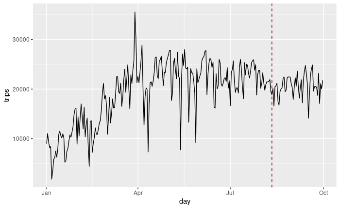
year_df %>% 
  ggplot(aes(x = day, y = trips)) + 
    geom_line() +
    geom_vline(xintercept = as.Date("2025-08-11"), linetype = "dashed", color = "darkred")

Recent Ridership Trend

Zooming into just this summer gives us a cleaner visual sense of the impact, albeit without perfectly clear answers either. This trend seems to show trip activity starting to decline just a bit before the August 11th announcements (perhaps in anticipation?), and then reaching a low point about a week after. Subsequently, ridership seems to have rebounded in September, but remains below the July steady-state level.

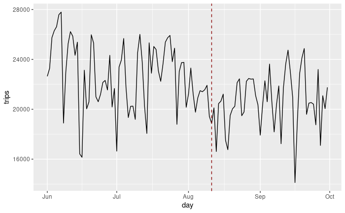
recent_df %>% 
  ggplot(aes(x = day, y = trips)) + 
    geom_line() +
    geom_vline(xintercept = as.Date("2025-08-11"), linetype = "dashed", color = "darkred")

Changepoint Detection

Applying the changepoint library to the trend is an easy way to see if we can automatically deduce the time at which behavior changed.

Running against our data, we can confirm that there is a changepoint around the time of August 11th - notably, happening just slightly before. This is an interesting indication that seems to imply that the “chilling” of activity in the city actually started about a week before… which intersects well with the Administration’s use of federal law enforcement officers to patrol Washington, DC on August 7th.

I thought this finding was super interesting as it implies that the increased presence of federal agents is what kickstarted the ridership decline - it’s not like the trend was stable until the August 11th National Guard deployment.

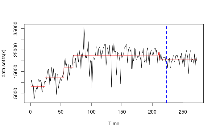
library(changepoint)

cp_mv <- cpt.meanvar(year_df %>% pull(trips), method = "PELT", penalty = "BIC")

plot(cp_mv)
abline(v = as.numeric(as.Date("2025-08-11") - min(year_df$day)) + 1,
       col = "blue", lwd = 2, lty = 2)

Interrupted Time Series (ITS) Regression

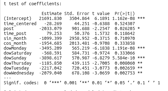
To quantify the ridership impact that the changepoints and visual trends point towards, we can use an interrupted time series regression model. Our model de-seasonalizes the trends for day of week and month of year effects and then provides a coefficient for the impact of post, a dummy variable which aggregates the rough impact of a day being the in the post-August 11th period.

We’ll exclude the intermediate period from August 7th to 11th, and focus on comparing the “pre-enforcement” period prior to August 7th against the “post-enforcement” period starting August 11th, where all the actions in the city were live.

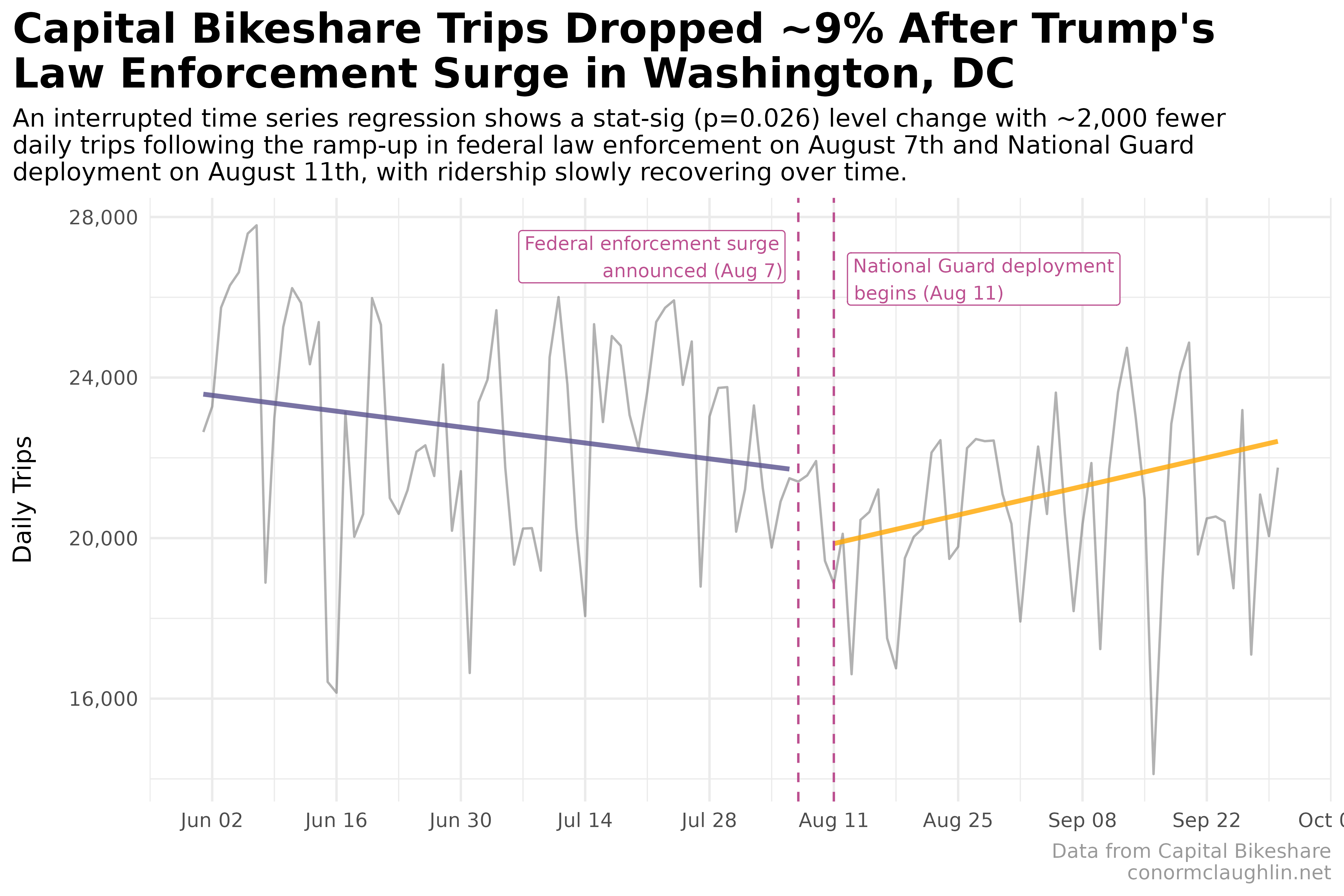
We find that post has an estimated value of -2,033 and p-value of 0.026, which tells us not only that the post-period saw a decline of rides to the tune of two thousand per day, but that the decline is statistically significant and unlikely to be noise.

library(tidyverse)
library(lmtest)
library(sandwich)
library(scales)

# have the "pre" period end Aug 7th and "post" start Aug 11th
cut_pre  <- as.Date("2025-08-07")  # end of "pre" period (exclusive)
cut_post <- as.Date("2025-08-11")  # start of "post" period (inclusive)

# exclude the days between the pre and post and engineer timeseries features
df_src <- recent_df

df_filtered <- df_src %>%
  mutate(day = as.Date(day)) %>%
  filter(day < cut_pre | day >= cut_post) %>%  
  mutate(
    # center time on Aug 7
    time_centered = as.numeric(day - cut_pre),
    post          = as.integer(day >= cut_post),
    time_post     = time_centered * post,
    # include timeseries features to help control regression for seasonality
    dow           = factor(weekdays(day)),
    month_num     = as.numeric(format(day, "%m")),
    sin_month     = sin(2 * pi * month_num / 12),
    cos_month     = cos(2 * pi * month_num / 12)
  )

# fit the timeseries using features
model_gap <- lm(
  trips ~ time_centered + post + time_post + sin_month + cos_month + dow,
  data = df_filtered
)

# output model details and coefficients
coeftest(model_gap, vcov = NeweyWest(model_gap, lag = 7))

Putting it all Together

Earlier I said I would look at:

1. If there IS any identifiable change in ridership associated with the August 11th law enforcement changes
2. IF SO, to what degree behavior has changed and whether or not things have rebounded since or remained depressed

Our data gives us clear and interesting answers:

1. There was a clear and statistically significant change in ridership associated with the ramp-up in law enforcement in the District. However, the data seem to show the decline actually started on August 7th, coincident with the increase of Federal law enforcement agents, rather than August 11th and the deployment of National Guard troops
2. If we compare the post-August 11th landscape against the pre-August 7th environment, we find there was an immediate step-down of roughly 2,000 daily trips, followed by a slow rebound back towards what I can assume is normality