A week ago, LeBron made his season debut for the Lakers, posting an 11/3/12 line in 29 minutes against the Jazz. The outing was particularly notable because it marked the first time any NBA player has ever competed in their 23rd season - a remarkable feat of longevity.
A few days later, I found myself watching the Washington Wizards at my parents’ house in an “Emirates NBA Cup” match against the Atlanta Hawks. It was some pretty bad basketball, to be honest - but the extreme youth of the Wizards, especially given LeBron’s recent milestone, caught my eye.
After checking, I found that six players on the Wizards’ roster were born after LeBron’s debut on October 29, 2003!
Visualizing
The Wizards example made me curious about how many players across the entire league are “younger” than LeBron’s career and how that number has evolved over the last few seasons.
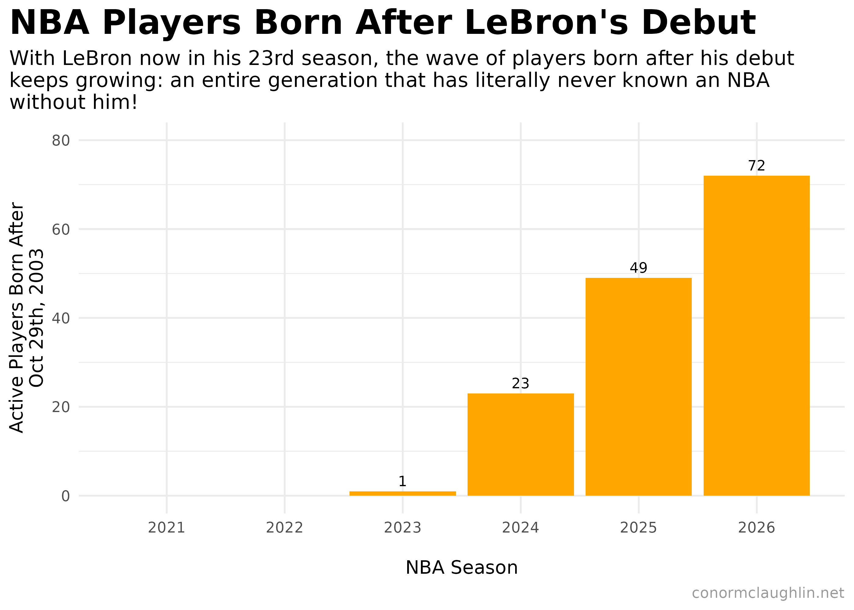
We find that 2023 was the first season with an active player born after LeBron’s debut, with Jalen Duren (who reclassified in high school) being the lone player. The number has increased quite a bit in the last two years, with 49 players last season and 72 players this season!
Code Reference
Fetch Player Box Scores by Season
library(hoopR)
library(tidyverse)

pbx <- load_nba_player_box(
  seasons = 2020:most_recent_nba_season()  # helper from hoopR
)

player_years <- pbx %>%
  group_by(season, athlete_id, athlete_display_name) %>%
  summarize(games = sum(minutes > 0, na.rm = TRUE))
Function to Fetch Player Date of Birth (DoB)
safe_get_player_dob <- function(athlete_id, year) {
  res <- tryCatch(
    espn_nba_player_stats(
      athlete_id = as.integer(athlete_id),   # ensure integer
      year       = year,
      season_type = "regular",
      total       = FALSE
    ),
    error = function(e) NULL
  )

  # If call fails or returns no rows, keep the structure but NA DOB
  if (is.null(res) || nrow(res) == 0) {
    return(tibble(
      espn_year  = year,
      birth_date = as.Date(NA_character_)
    ))
  }

  res %>%
    slice(1) %>%                # one row is enough
    transmute(
      espn_year  = year,
      birth_date = as.Date(date_of_birth)   # from espn_nba_player_stats docs
    )
}
Code to Look Up DoB per Player
player_bio <- player_years %>%
  distinct(athlete_id, season) %>%
  group_by(athlete_id) %>%
  summarize(first_season = min(season), .groups = "drop") %>%
  mutate(
    data = map2(athlete_id, first_season, safe_get_player_dob)
  ) %>%
  unnest(cols = data)
Join DoB Back to Season Logs
season_summary <- player_years %>%
  left_join(player_bio, by = "athlete_id") %>%
  filter(!is.na(birth_date)) %>%
  mutate(
    born_after_debut = birth_date > lebron_debut
  ) group_by(season) %>%
  summarize(
    n_unique_opponents_after = n_distinct(athlete_id[born_after_debut]),
    .groups = "drop"
  )
Build the Chart
season_summary %>% filter(season >= 2021) %>%
ggplot(aes(x = season, y = n_unique_opponents_after, label = ifelse(n_unique_opponents_after > 0, n_unique_opponents_after, NA))) +
  geom_col(fill = "#ffa600") +
  geom_text(vjust = -0.5, size = 3, face = "bold") +
  scale_x_continuous(breaks = scales::pretty_breaks(n = 8)) +
  scale_y_continuous(limits = c(0, 80), breaks = scales::pretty_breaks(n = 6)) +
  theme_minimal() +
  theme(
    panel.grid.minor.x = element_blank(),
    strip.background = element_rect(fill = "grey30"),
    strip.text = element_text(color = "grey97", face = "bold"),
    legend.background = element_rect(color = NA),
    plot.title = element_text(size = 20, face = "bold"),
    plot.subtitle = element_text(size = 12),
    plot.caption = element_text(colour = "grey60"),
    plot.title.position = "plot"
  ) +
  labs(
    x = "\nNBA Season",
    y = "Active Players Born After\nOct 29th, 2003",
    title = "NBA Players Born After LeBron's Debut",
    subtitle = "With LeBron now in his 23rd season, the wave of players born after his debut\nkeeps growing: an entire generation that has literally never known an NBA\nwithout him!",
    caption = "conormclaughlin.net"
  )