On May 2nd, Spirit Airlines permanently ceased operations. The airline, which had been the seventh-largest in the US, leaves behind 172 planes (many of which are currently being ferried back to their lessors) and 73 destinations.
It’s those destinations I’m most curious about - what will happen to them when Spirit exits?
While Spirit may have been a terminally flawed business, boxed out by labor costs and the “k-shaped” economic recovery following the pandemic, it did have a genuine role in the US aviation world as a low-fare spill carrier, keeping more premium competitors honest on cost and capacity. This role benefited American consumers, even if they didn’t fly on Spirit directly.
With this in mind, I spent some time mucking about the Bureau of Transportation Statistics T-100 data, which shows flight capacity and load factors, and DB1C data, which captures fares paid. In this post, you’ll see visualizations from both datasets, seeking to shed light on Spirit’s operations at a high level.
Where was Spirit Flying?
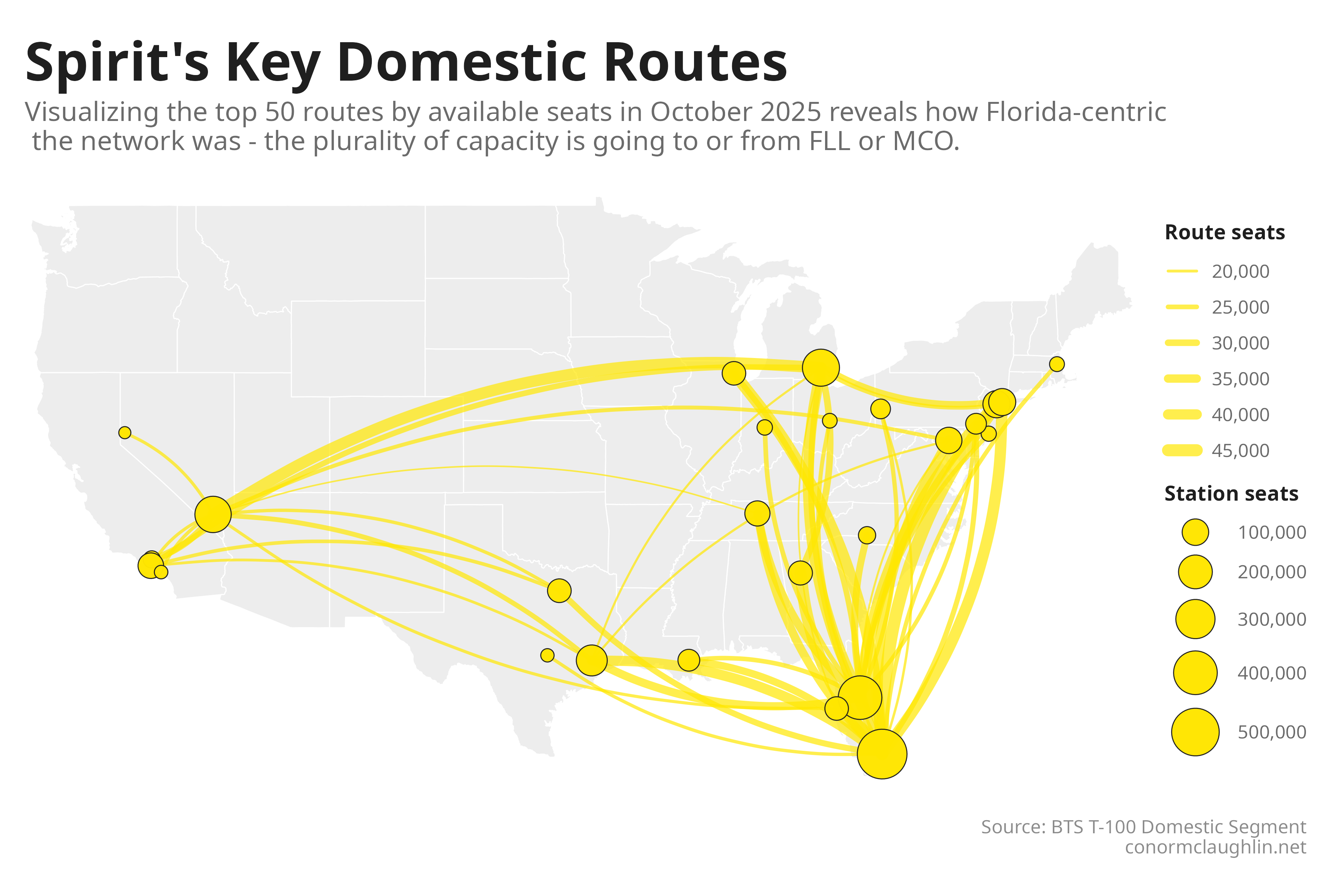
Starting with a map visualization drives home a key point to start off - while it might have dabbled in flying between major cities, Spirit was really a leisure airline at the end of the day, with a core competency of flying people to Florida.
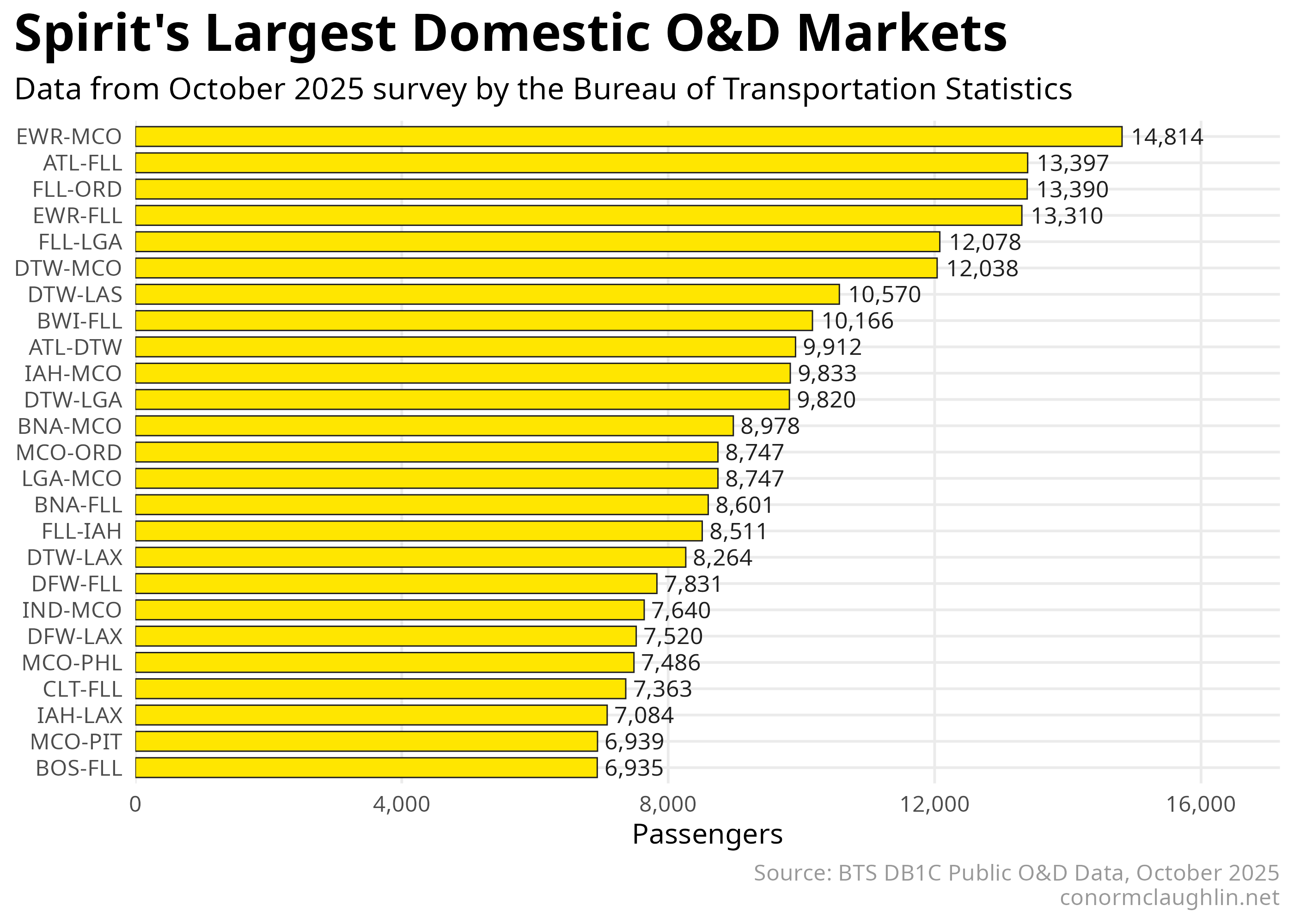
This trend is clearly visible when we look at the busiest O&D (origin and destination) markets, the vast majority of which touch either Fort Lauderdale (FLL) or Orlando (MCO).
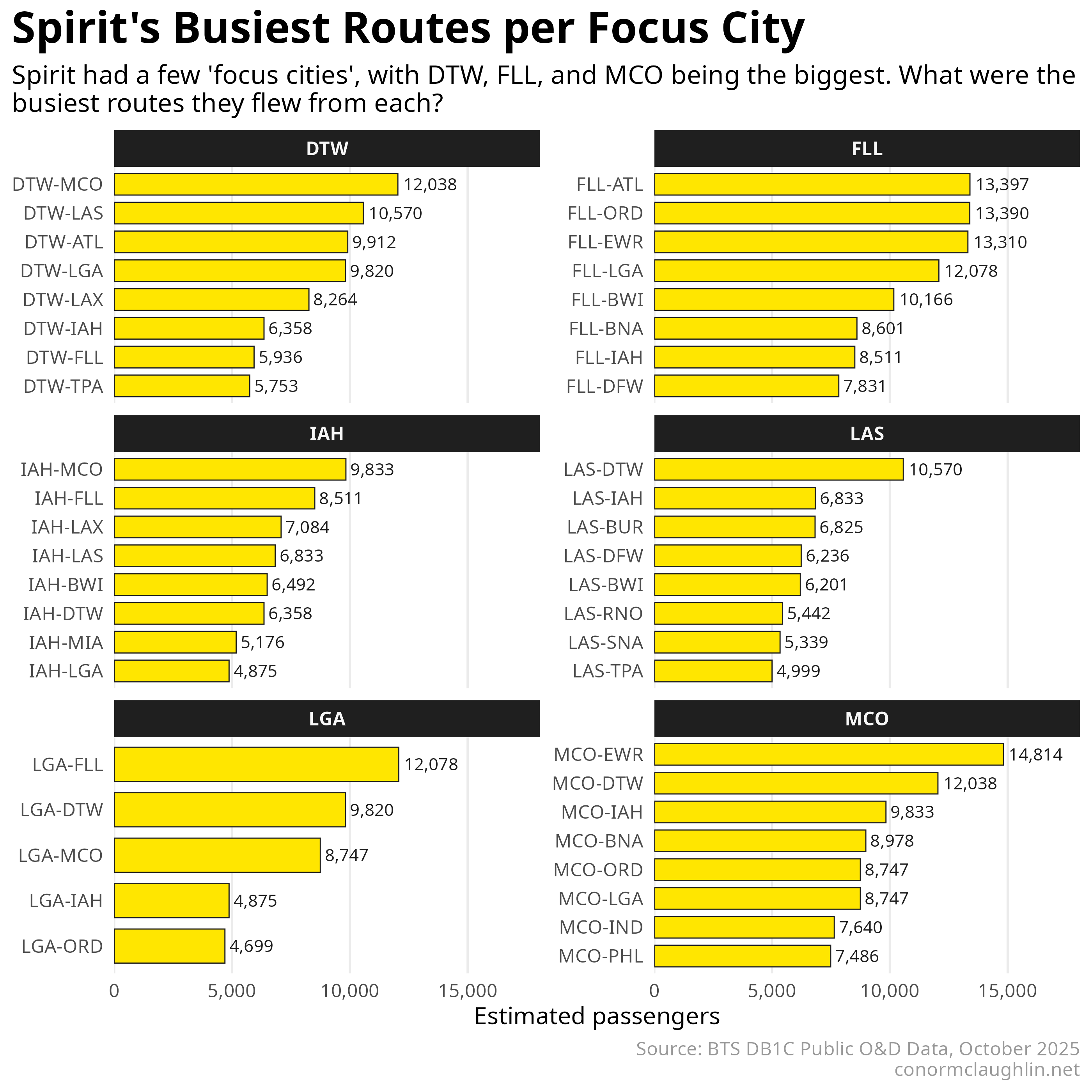
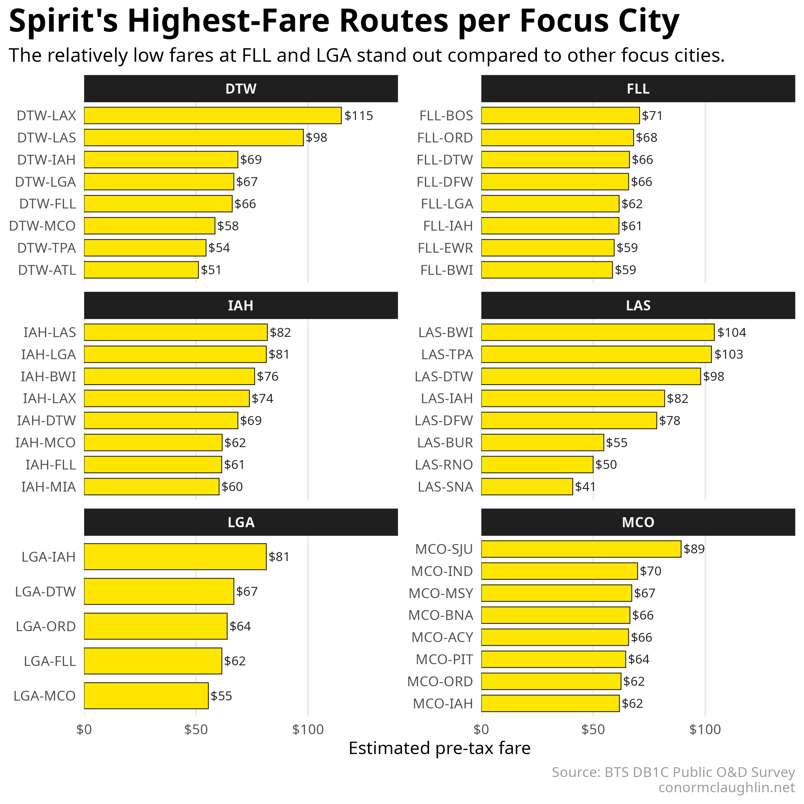
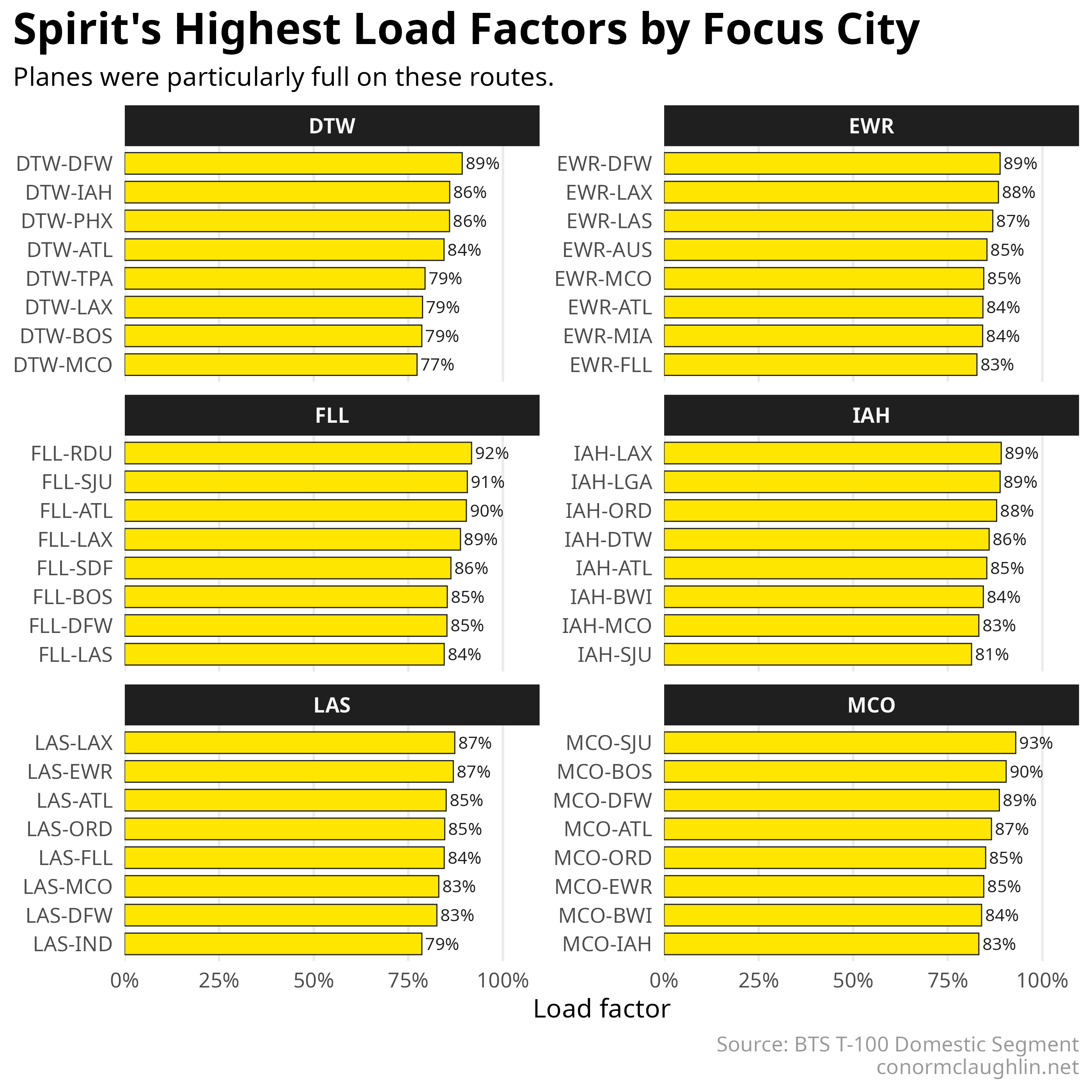
Breaking the data out by focus city makes everything a bit more legible…
What Might Other Airlines Backfill?
The Highest Fare Routes?
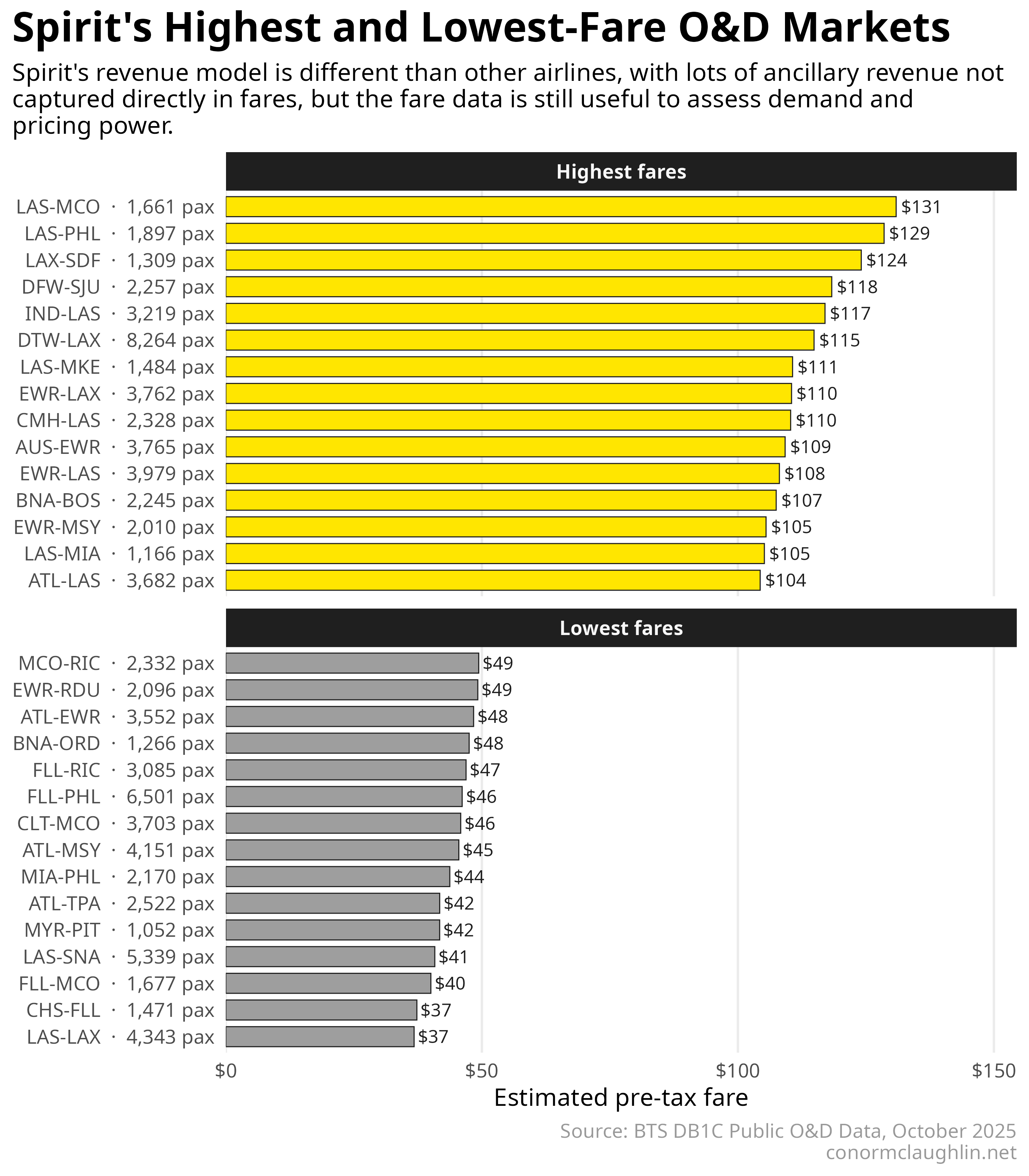
The DB1C data is awesome because it gives us a sense of the fares that customers are paying to fly between two markets. While in Spirit’s case, that may not represent the fully-loaded travel cost (since it was totally possible and maybe even probable to spend more on bags and seat assignments than the base fare itself), I think it’s a useful enough proxy to identify the high and low-potential routes within the network portfolio, that other airlines might want to go after.
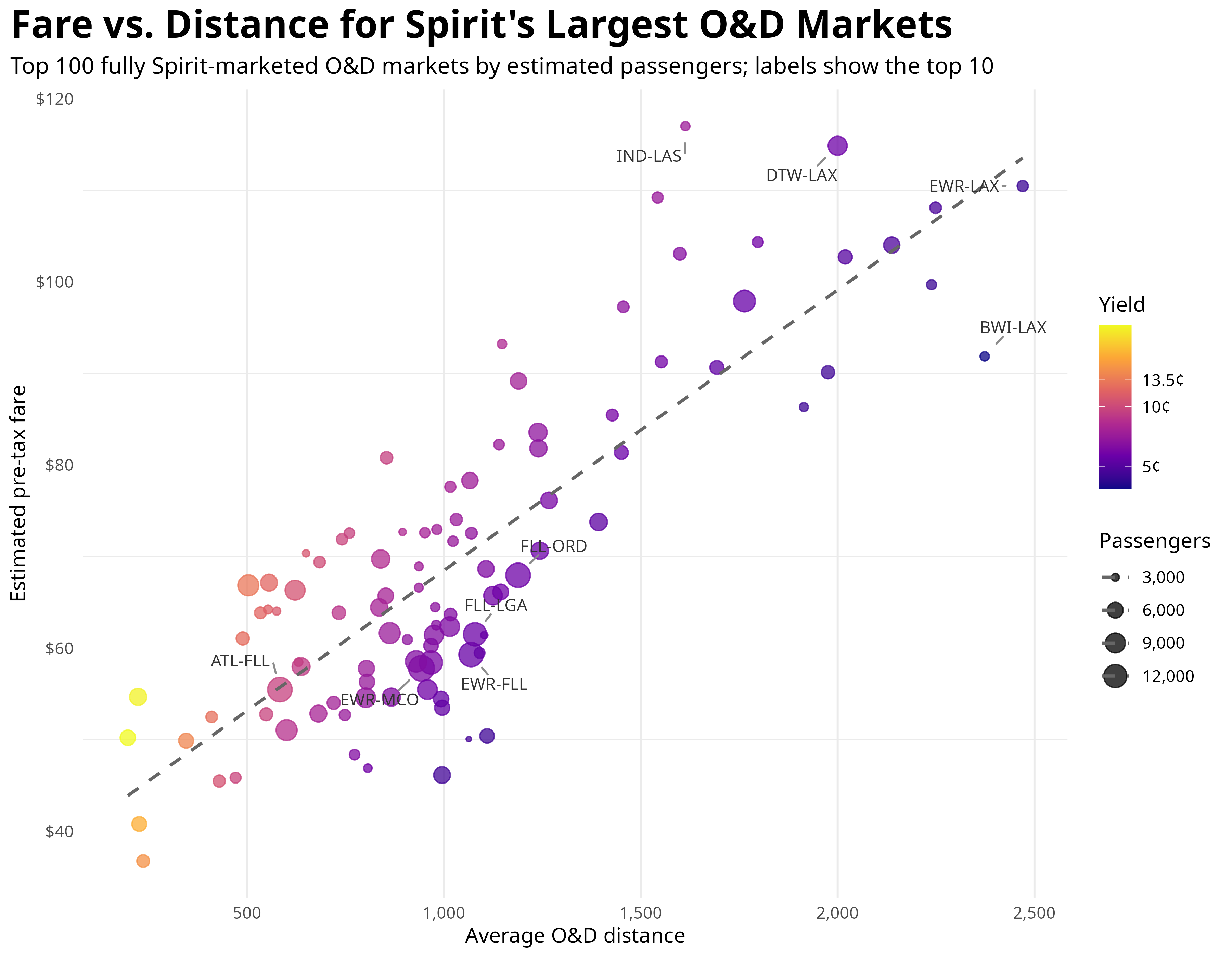
Plotting fares against distance flown starts to show the limits of this approach though - fares were generally a function of distance flown, and without knowing how many fares were actually sold, it’s hard to know if the flights were full enough to make money.
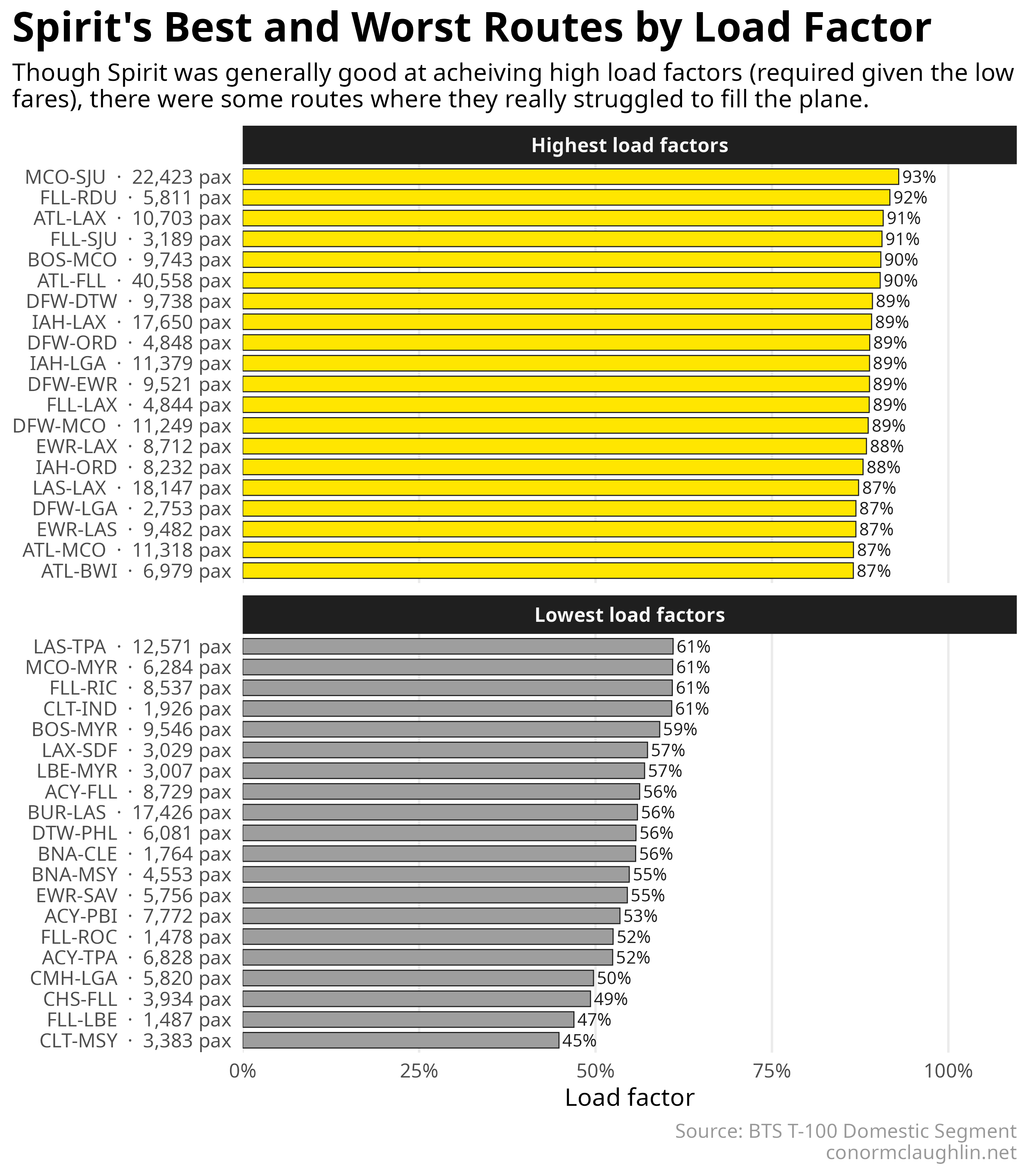
The Most Sold-Out Routes?
Fortunately for us, the BTS’s T-100 data provides load factors per flight, which supplies the additional angle we are looking for. Where was Spirit able to fully sell out their cabins, versus routes which were perennially half-empty?
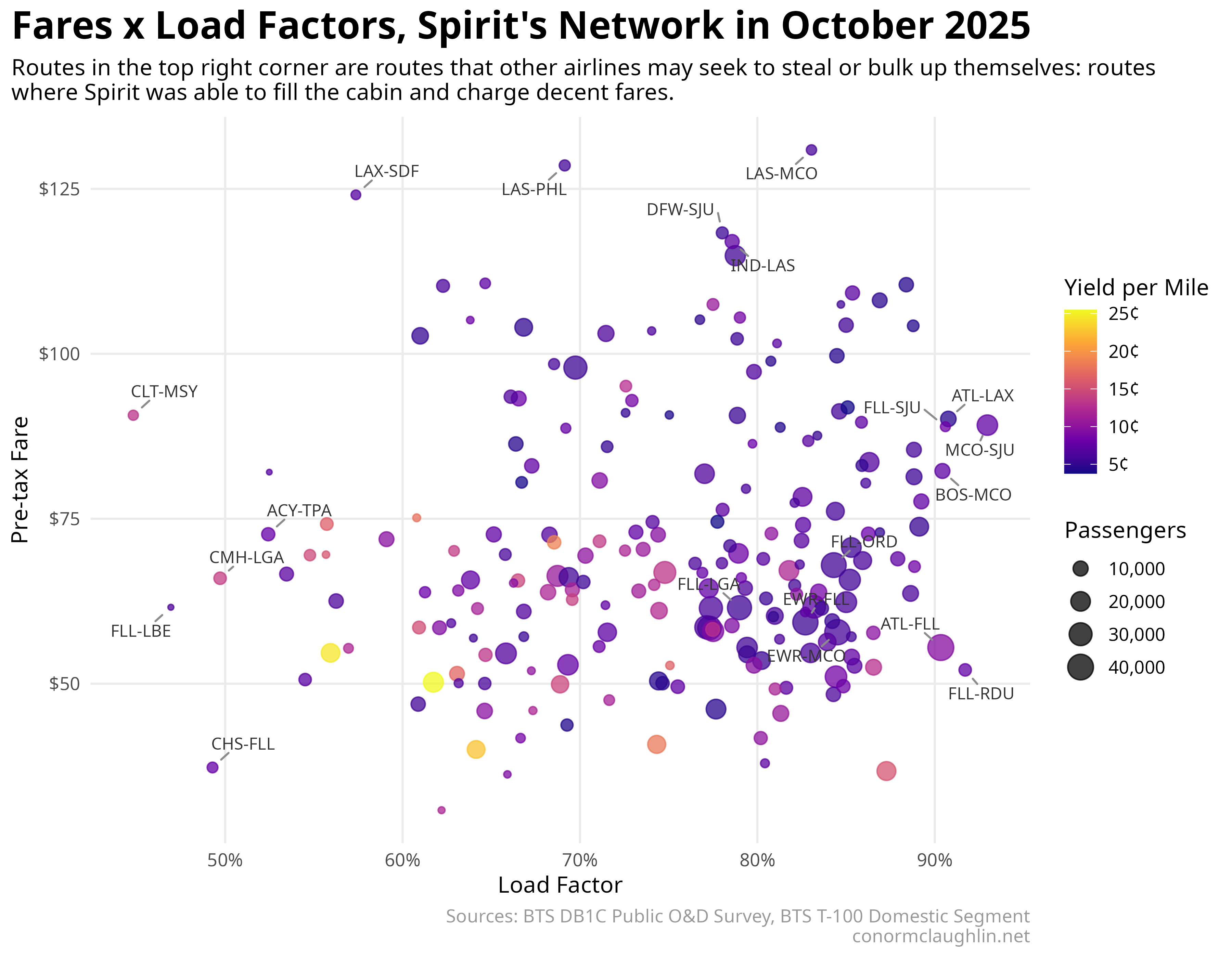
Or Both - Routes with High Fares and Load Factors?
Combining the DB1C data with the T-100 data gives us a fully unified dataset, and allows us to compare load factors and fares in a single view.
My best guess is that the other major US airlines will immediately step up frequencies for the Spirit flights in the top right quadrant of the chart: flights with full cabins and relatively high fares. JetBlue seems to have already kick-started this process in FLL…. I will be curious to see what carriers are best positioned to pick up the best routes out of MCO (no hub incumbent) and LAS (perhaps Southwest?!).
In Memoriam
One last thing - I will never, ever stop enjoying this photo of The Great Seafood Feast - perhaps the perfect embodiment of Spirit as a carrier, and also the reason for its downfall. RIP!

Code Reference
This was the second or third time I’ve run into a dataset too heavy to manipulate within R session memory… to make the data workable in my usual RStudio environment, I used Apache Arrow to lazy-load the columnar parquet data and DuckDB as a database engine. that stack makes working with medium-sized data trivial!
Loading the DB1C Data
library(arrow)
library(tidyverse)

# point to your file
path <- "DB1C.PUBLIC.202510.REL02.27FEB2026/DB1C.PUBLIC.202510.REL02.27FEB2026.parquet"

# lazy load (does NOT pull all into memory yet)
db1c <- open_dataset(path)
library(DBI)
library(duckdb)
library(glue)
library(scales)
library(stringr)

con <- dbConnect(duckdb())

duckdb_register_arrow(con, "db1c", db1c)

dir.create("~/duckdb_tmp", showWarnings = FALSE)

DBI::dbExecute(con, "SET preserve_insertion_order = false")
DBI::dbExecute(con, "SET temp_directory = '~/duckdb_tmp'")
DBI::dbExecute(con, "SET memory_limit = '6GB'")
DBI::dbExecute(con, "SET threads = 4")


# Fully Spirit-marketed itinerary filter:
# For every coupon that exists, MktCarrier_i must be NK.
all_spirit_where <- paste(
  sprintf("(CouponSeg < %s OR MktCarrier_%s = 'NK')", 1:23, 1:23),
  collapse = "\n  AND "
)

# Only keep columns needed downstream
# Important: Dwell_Time and TripBk fields start at _2, not _1

needed_cols <- c(
  "RpCarrier", "RpYear", "RpMonth", "CouponSeg", "IssueCarrier",
  "TotalAmt", "TaxAmt", "DollarCred", "NumPax", "PurWinGrp",

  unlist(lapply(1:23, function(i) {
    c(
      paste0("SchFlYr_", i),
      paste0("SchFlMo_", i),
      paste0("Apt_", i),
      paste0("CityMktID_", i),
      if (i == 1) "WAC_1" else paste0("CityWAC_", i),
      paste0("ViaApt_", i),
      paste0("OpCarrier_", i),
      paste0("MktCarrier_", i),
      paste0("Coupon_SegDist_", i)
    )
  })),

  # These start at _2 in your schema
  paste0("Dwell_Time_", 2:23),
  paste0("TripBk19_7_", 2:23),
  paste0("TripBk19_8_", 2:23),

  # Final destination fields
  "LastApt", "LastCityMktID", "LastCityWAC",
  "TripBk19_7_last", "TripBk19_8_last"
)

needed_cols <- unique(needed_cols)
needed_cols_sql <- paste(needed_cols, collapse = ",\n  ")


# This should be much smaller than scanning/materializing the full DB1C.
# RpCarrier = 'NK' is the big speedup.
DBI::dbExecute(con, glue("
CREATE OR REPLACE TABLE db1c_spirit_base AS
SELECT
  {needed_cols_sql}
FROM db1c
WHERE RpCarrier = 'NK'
  AND CouponSeg BETWEEN 1 AND 23
  AND {all_spirit_where}
"))


# Add ticket_id only after aggressive filtering
DBI::dbExecute(con, "
CREATE OR REPLACE TABLE db1c_spirit_base_numbered AS
SELECT
  row_number() OVER () AS ticket_id,
  *
FROM db1c_spirit_base
")

make_segment_sql <- function(i) {

  origin_airport <- paste0("Apt_", i)
  dest_airport   <- if (i < 23) paste0("Apt_", i + 1) else "LastApt"

  origin_city <- paste0("CityMktID_", i)
  dest_city   <- if (i < 23) paste0("CityMktID_", i + 1) else "LastCityMktID"

  origin_wac <- if (i == 1) "WAC_1" else paste0("CityWAC_", i)
  dest_wac   <- if (i < 23) paste0("CityWAC_", i + 1) else "LastCityWAC"

  trip_break_197 <- if (i < 23) paste0("TripBk19_7_", i + 1) else "TripBk19_7_last"
  trip_break_198 <- if (i < 23) paste0("TripBk19_8_", i + 1) else "TripBk19_8_last"

  dwell_after <- if (i < 23) paste0("Dwell_Time_", i + 1) else "NULL"

  glue("
    SELECT
      ticket_id,

      RpCarrier,
      RpYear,
      RpMonth,
      CouponSeg,
      IssueCarrier,
      TotalAmt,
      TaxAmt,
      DollarCred,
      NumPax,
      PurWinGrp,

      {i} AS segment_no,

      SchFlYr_{i} AS sch_flight_year,
      SchFlMo_{i} AS sch_flight_month,

      {origin_airport} AS origin_airport,
      {dest_airport} AS dest_airport,

      {origin_city} AS origin_city_market_id,
      {dest_city} AS dest_city_market_id,

      {origin_wac} AS origin_wac,
      {dest_wac} AS dest_wac,

      ViaApt_{i} AS via_airport,
      OpCarrier_{i} AS op_carrier,
      MktCarrier_{i} AS mkt_carrier,

      Coupon_SegDist_{i} AS segment_distance,
      {dwell_after} AS dwell_time_after,

      {trip_break_197} AS trip_break_197,
      {trip_break_198} AS trip_break_198

    FROM db1c_spirit_base_numbered
    WHERE CouponSeg >= {i}
      AND {origin_airport} IS NOT NULL
      AND {dest_airport} IS NOT NULL
  ")
}

segment_sql <- paste(
  vapply(1:23, make_segment_sql, character(1)),
  collapse = "\nUNION ALL\n"
)


DBI::dbExecute(con, glue("
CREATE OR REPLACE TEMP TABLE db1c_segments AS
WITH base AS (
  SELECT
    row_number() OVER () AS ticket_id,
    *
  FROM db1c_spirit_base_numbered
)
{segment_sql}
"))
Turning the Segments into O&D Trips
DBI::dbExecute(con, "
CREATE OR REPLACE TEMP TABLE db1c_od_trips AS
WITH marked AS (
  SELECT
    *,
    CASE
      WHEN trip_break_197 IN ('X', 'Y') THEN 1
      WHEN segment_no = CouponSeg THEN 1
      ELSE 0
    END AS ends_trip
  FROM db1c_segments
),

numbered AS (
  SELECT
    *,
    1 + COALESCE(
      SUM(ends_trip) OVER (
        PARTITION BY ticket_id
        ORDER BY segment_no
        ROWS BETWEEN UNBOUNDED PRECEDING AND 1 PRECEDING
      ),
      0
    ) AS trip_no
  FROM marked
),

ticket_totals AS (
  SELECT
    ticket_id,
    SUM(segment_distance) AS itinerary_distance
  FROM db1c_segments
  GROUP BY ticket_id
),

trip_rollup AS (
  SELECT
    ticket_id,
    trip_no,

    ANY_VALUE(RpCarrier) AS reporting_carrier,
    ANY_VALUE(RpYear) AS report_year,
    ANY_VALUE(RpMonth) AS report_month,
    ANY_VALUE(CouponSeg) AS coupon_segments,
    ANY_VALUE(IssueCarrier) AS issue_carrier,
    ANY_VALUE(PurWinGrp) AS purchase_window_group,

    ANY_VALUE(TotalAmt) AS total_amount,
    ANY_VALUE(TaxAmt) AS tax_amount,
    ANY_VALUE(NumPax) AS num_pax,

    FIRST(origin_airport ORDER BY segment_no) AS origin_airport,
    LAST(dest_airport ORDER BY segment_no) AS dest_airport,

    FIRST(origin_city_market_id ORDER BY segment_no) AS origin_city_market_id,
    LAST(dest_city_market_id ORDER BY segment_no) AS dest_city_market_id,

    FIRST(origin_wac ORDER BY segment_no) AS origin_wac,
    LAST(dest_wac ORDER BY segment_no) AS dest_wac,

    COUNT(*) AS n_segments,
    SUM(segment_distance) AS trip_distance,

    FIRST(origin_airport ORDER BY segment_no) || '-' ||
      STRING_AGG(dest_airport, '-' ORDER BY segment_no) AS path,

    BOOL_OR(mkt_carrier = 'NK') AS any_mkt_spirit,
    BOOL_AND(mkt_carrier = 'NK') AS all_mkt_spirit,

    BOOL_OR(op_carrier = 'NK') AS any_op_spirit,
    BOOL_AND(op_carrier = 'NK') AS all_op_spirit,

    STRING_AGG(DISTINCT mkt_carrier, ',') AS mkt_carriers,
    STRING_AGG(DISTINCT op_carrier, ',') AS op_carriers

  FROM numbered
  GROUP BY ticket_id, trip_no
)

SELECT
  tr.*,
  tt.itinerary_distance,

  CASE
    WHEN tr.tax_amount IS NULL THEN tr.total_amount
    ELSE tr.total_amount - tr.tax_amount
  END AS base_fare_est,

  CASE
    WHEN tt.itinerary_distance > 0 THEN
      (
        CASE
          WHEN tr.tax_amount IS NULL THEN tr.total_amount
          ELSE tr.total_amount - tr.tax_amount
        END
      ) * tr.trip_distance / tt.itinerary_distance
    ELSE NULL
  END AS allocated_base_fare,

  CASE
    WHEN tr.origin_airport < tr.dest_airport THEN tr.origin_airport || '-' || tr.dest_airport
    ELSE tr.dest_airport || '-' || tr.origin_airport
  END AS route,

  tr.origin_airport || '-' || tr.dest_airport AS directional_route,

  CASE
    WHEN tr.n_segments = 1 THEN TRUE
    ELSE FALSE
  END AS nonstop_trip,

  CASE
    WHEN tr.n_segments > 1 THEN TRUE
    ELSE FALSE
  END AS connecting_trip

FROM trip_rollup tr
LEFT JOIN ticket_totals tt
  ON tr.ticket_id = tt.ticket_id
")
Compile Spirit Data at the Route Level
spirit_od_routes_all <- tbl(con, "db1c_od_trips") %>%
  filter(all_mkt_spirit) %>%
  mutate(
    passenger_miles = num_pax * trip_distance,
    fare_revenue_est = num_pax * allocated_base_fare,
    connecting_pax = case_when(
      connecting_trip ~ num_pax,
      TRUE ~ 0L
    ),
    nonstop_pax = case_when(
      nonstop_trip ~ num_pax,
      TRUE ~ 0L
    )
  ) %>%
  group_by(route) %>%
  summarise(
    passengers = sum(num_pax, na.rm = TRUE),
    tickets = n(),
    fare_revenue_est = sum(fare_revenue_est, na.rm = TRUE),
    passenger_miles = sum(passenger_miles, na.rm = TRUE),
    connecting_pax = sum(connecting_pax, na.rm = TRUE),
    nonstop_pax = sum(nonstop_pax, na.rm = TRUE),
    distance_weighted = sum(trip_distance * num_pax, na.rm = TRUE),
    fare_weighted = sum(allocated_base_fare * num_pax, na.rm = TRUE),
    segments_weighted = sum(n_segments * num_pax, na.rm = TRUE),
    .groups = "drop"
  ) %>%
  mutate(
    avg_distance = distance_weighted / passengers,
    avg_fare = fare_weighted / passengers,
    avg_segments = segments_weighted / passengers,
    yield_est = fare_revenue_est / passenger_miles,
    connecting_share = connecting_pax / passengers,
    nonstop_share = nonstop_pax / passengers
  ) %>%
  select(
    route,
    passengers,
    tickets,
    fare_revenue_est,
    avg_fare,
    yield_est,
    avg_distance,
    avg_segments,
    nonstop_share,
    connecting_share,
    passenger_miles
  ) %>%
  arrange(desc(passengers))


top_spirit_routes_by_passengers <- spirit_od_routes_all %>%
  head(50) %>%
  collect()

top_spirit_routes_by_revenue <- spirit_od_routes_all %>%
  arrange(desc(fare_revenue_est)) %>%
  head(50) %>%
  collect()

top_spirit_routes_by_yield <- spirit_od_routes_all %>%
  filter(passengers >= 1000) %>%
  arrange(desc(yield_est)) %>%
  head(50) %>%
  collect()
Visualization
# ------------------------------------------------------------------------------
# Highest and lowest Spirit O&D markets by average fare
# ------------------------------------------------------------------------------

library(forcats)
library(scales)
library(ggplot2)
library(dplyr)

spirit_yellow <- "#FFE600"
spirit_black  <- "#1F1F1F"
spirit_grey   <- "#6B6B6B"
low_fare_grey <- "#9E9E9E"

min_passengers <- 1000
n_routes <- 15

spirit_fare_extremes <- spirit_od_routes_all %>%
  filter(passengers >= min_passengers) %>%
  collect()

top_fares <- spirit_fare_extremes %>%
  slice_max(avg_fare, n = n_routes) %>%
  mutate(fare_group = "Highest fares")

low_fares <- spirit_fare_extremes %>%
  slice_min(avg_fare, n = n_routes) %>%
  mutate(fare_group = "Lowest fares")

fare_extremes <- bind_rows(top_fares, low_fares) %>%
  mutate(
    fare_group = factor(fare_group, levels = c("Highest fares", "Lowest fares")),
    route_label = paste0(route, "  ·  ", comma(passengers), " pax"),
    route_label = fct_reorder(route_label, avg_fare)
  )

ggplot(
  fare_extremes,
  aes(x = avg_fare, y = route_label, fill = fare_group)
) +
  geom_col(
    color = spirit_black,
    linewidth = 0.25,
    width = 0.75
  ) +
  geom_text(
    aes(label = dollar(avg_fare, accuracy = 1)),
    hjust = -0.12,
    size = 3.1,
    color = spirit_black
  ) +
  facet_wrap(
    ~ fare_group,
    scales = "free_y",
    ncol = 1
  ) +
  scale_fill_manual(
    values = c(
      "Highest fares" = spirit_yellow,
      "Lowest fares" = low_fare_grey
    )
  ) +
  scale_x_continuous(
    labels = dollar_format(),
    expand = expansion(mult = c(0, 0.18))
  ) +
  theme_minimal(base_size = 12) +
  theme(
    panel.grid.minor.x = element_blank(),
    panel.grid.major.y = element_blank(),
    strip.background = element_rect(fill = spirit_black, color = NA),
    strip.text = element_text(color = "grey97", face = "bold"),
    legend.position = "none",
    legend.background = element_rect(color = NA),
    plot.title = element_text(size = 20, face = "bold"),
    plot.subtitle = element_text(size = 12),
    plot.caption = element_text(colour = "grey60"),
    plot.title.position = "plot"
  ) +
  labs(
    title = "Spirit's Highest and Lowest-Fare O&D Markets",
    subtitle = "Spirit's revenue model is different than other airlines, with lots of ancillary revenue not\ncaptured directly in fares, but the fare data is still useful to assess demand and\npricing power.",
    x = "Estimated pre-tax fare",
    y = NULL,
    caption = "Source: BTS DB1C Public O&D Data, October 2025\nconormclaughlin.net"
  )